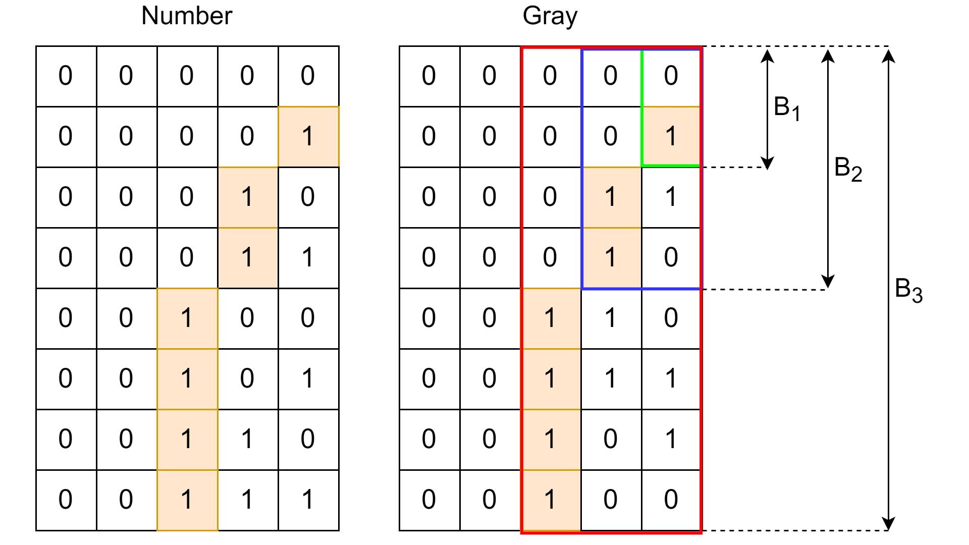
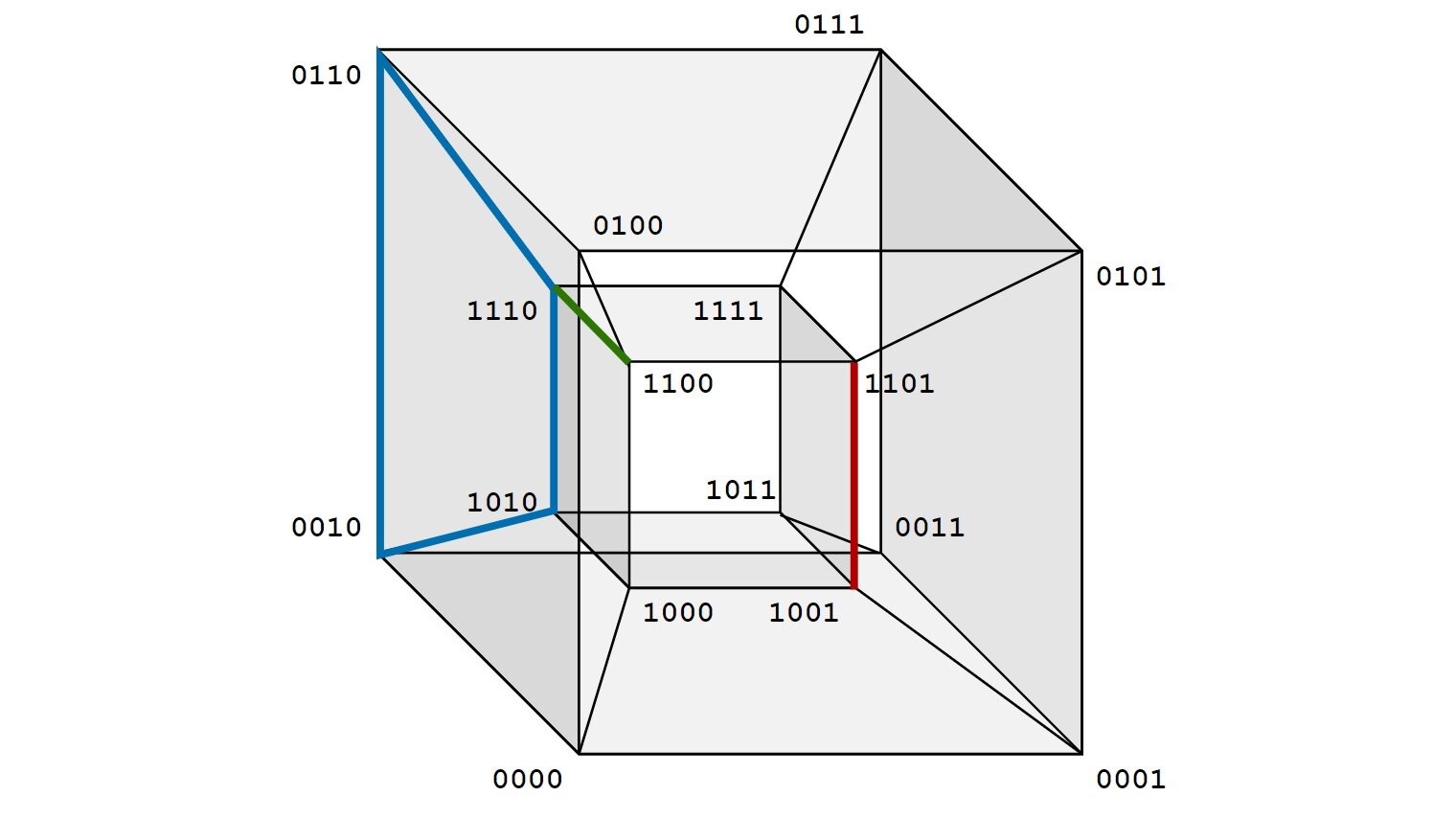
This post is about gray codes a.k.a. gray encoding of binary numbers. We will also cover some interesting properties, ideas and symmetries behind this encoding.
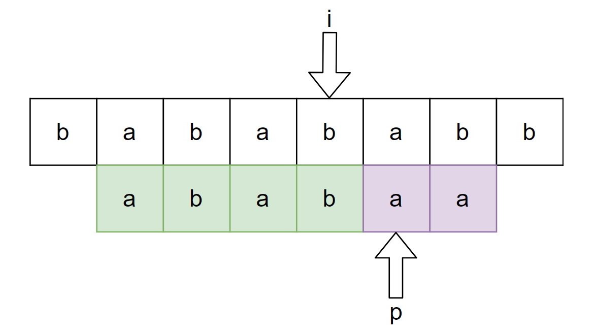
Almost every program has to somehow process and transform strings. Very often we want to identify some fixed pattern (substring) in the string, or, formally speaking, find an occurrence of β:=b0b1…bn−1 in α:=a0a1…am−1=ε. A naive algorithm would just traverse α and check if β starts at the current character of α. Unfortunately, this approach leads us to an algorithm with a complexity of O(n⋅m). In this post we will discuss a more efficient algorithm solving this problem - the Knuth-Morris-Pratt (KMP) algorithm.
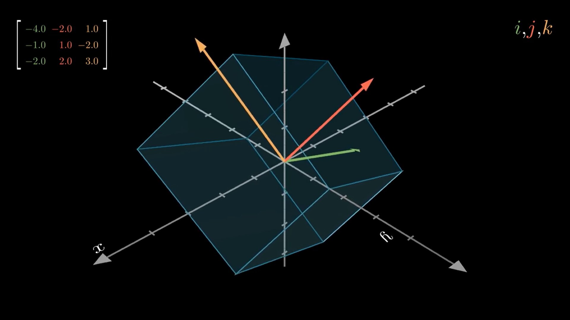
Matrices are omnipresent in linear algebra. Columns of a matrix describe where the corresponding basis vectors land relative to the initial basis. All transformed vectors are linear combinations of transformed basis vectors which are the columns of the matrix, this is also called linearity. Algorithms that operate on matrices essentially just alter the way vectors get transformed, preserving some properties. Unfortunately, many algorithms are typically presented to students in a numerical fashion, without describing the whole graphical meaning. In this post we will first visualize simple linear transformations and then we will visualize Gaussian Elimination (with row swaps) steps as a sequence of linear transformations. To do this, we will use Python together with a popular Open-Source library manim.
Linear systems of equations come up in almost any technical discipline. The PA=LU factorization method is a well-known numerical method for solving those types of systems of equations against multiple input vectors. It is also possible to preserve numerical stability by implementing some pivot strategy. In this post we will consider performance and numerical stability issues and try to cope with them by using the PA = LU factorization.
In this post we will examine an interesting connection between the NP-complete CNF-SAT problem and the problem of computing the amount of words generated by some efficient representation of a formal language. Here, I call a way of representing a formal language efficient, if it has a polynomially-long encoding but can possibly describe an exponentially-large formal language. Examples of such efficient representations are nondeteministic finite automations and regular expressions.
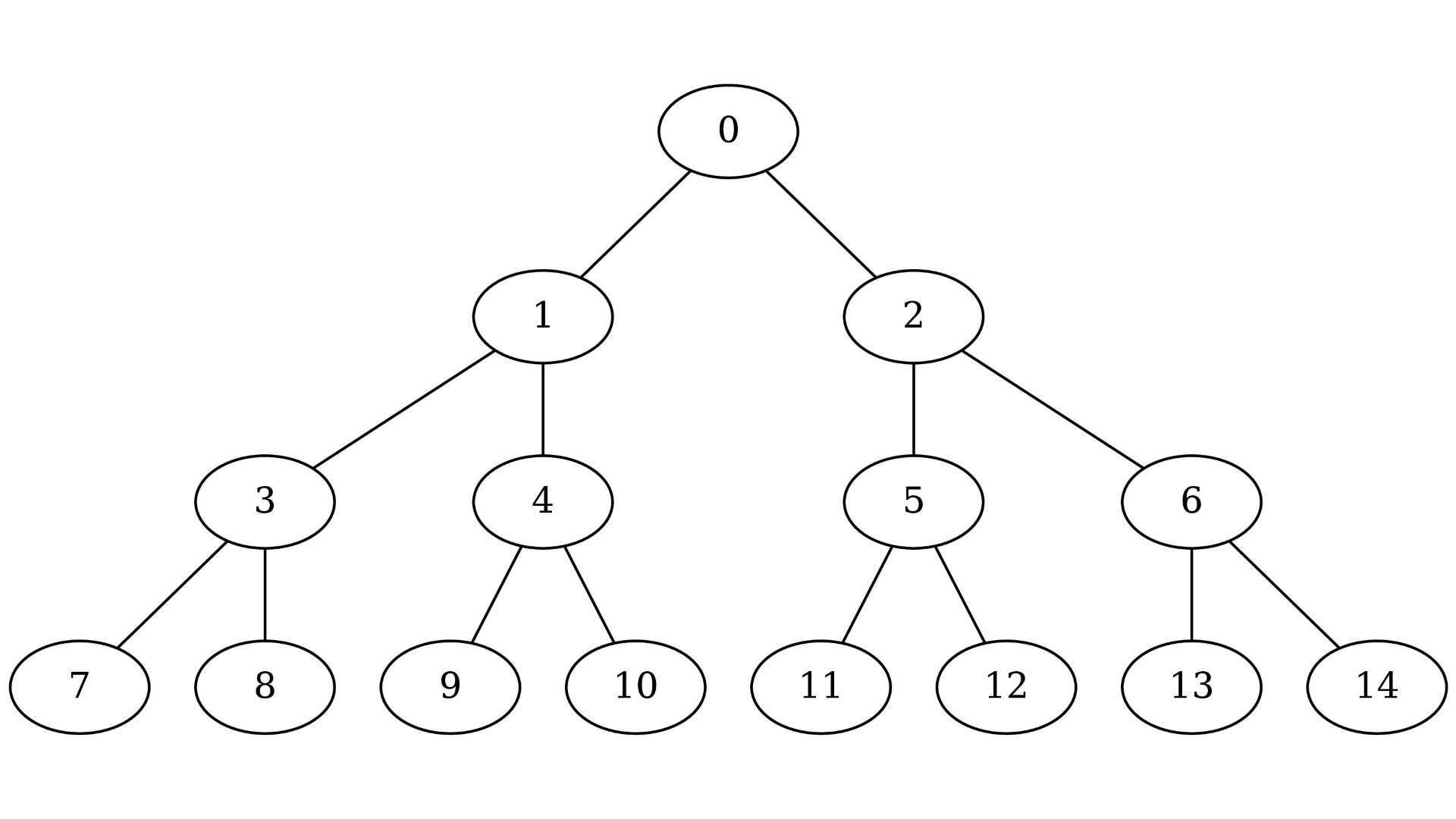
The lowest common ancestor (LCA) problem is important in many applications of binary trees. For example, by knowing the lowest common ancestor we can easily compute the shortest path between any two vertices in a tree. The most common way to compute the lca of vertices u and v is to iteratively go up until we get to the root of the subtree containing both u and v. This method works only if u and v are on the same level. If not, we can first measure the difference of heights d between u and v and then find the lowest common ancestor of the d-th parent of the lowest vertex and the higher vertex.
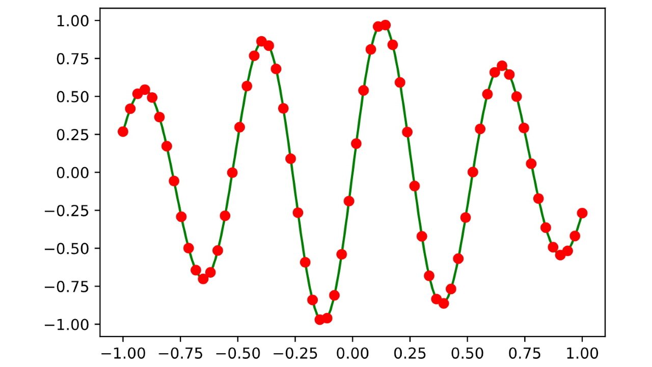
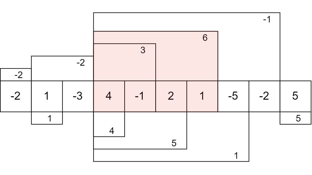
People often refer to Kadane’s algorithm only in the context of the maximum subarray problem. However, the idea behind this algorithm allows one to use it for solving a variety of problems that have something to do with finding a continuous subarray with a given property. The algorithm can also be used in 2d or multidimensional arrays but in this post we will only consider regular one-dimensional arrays.
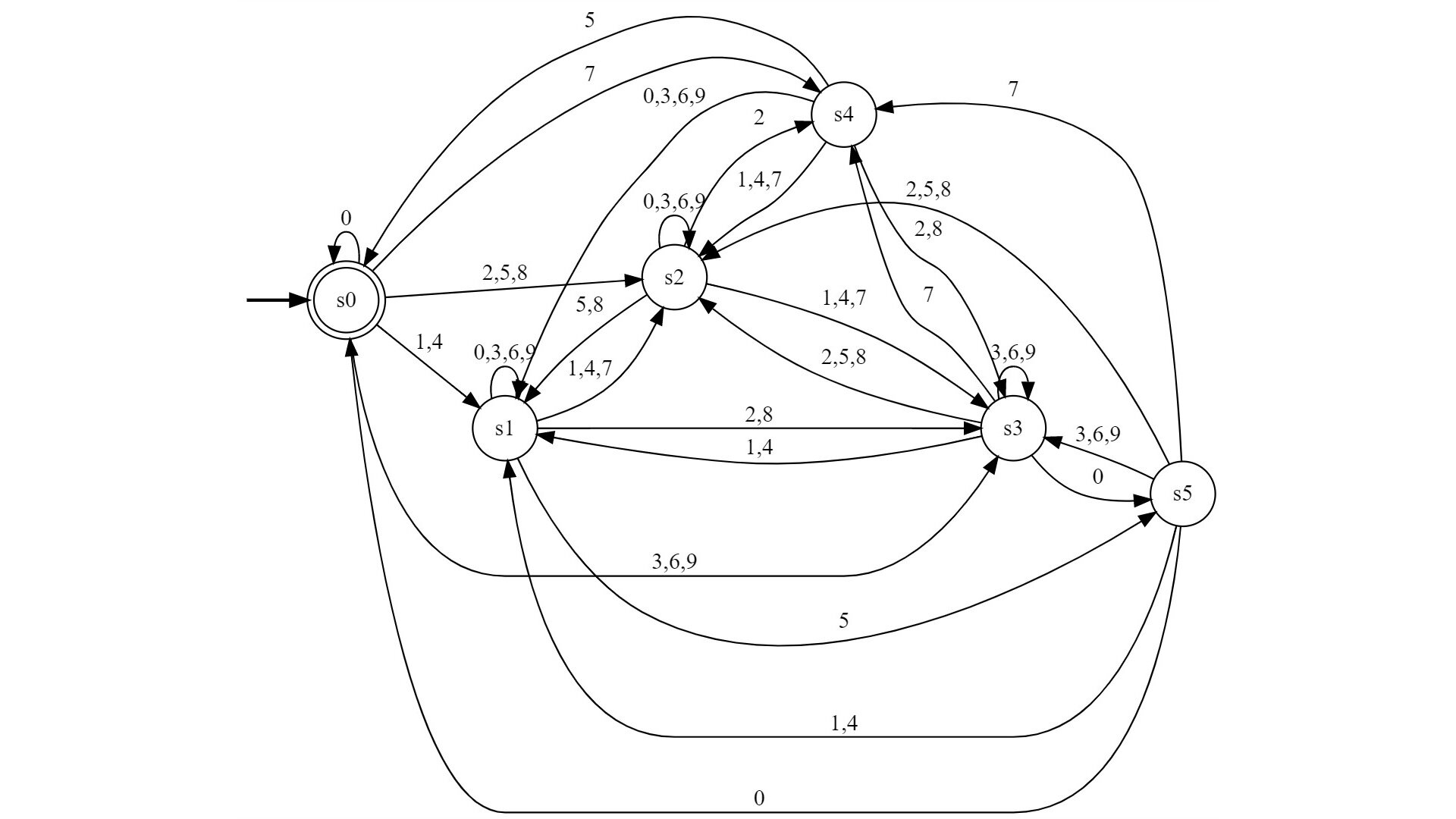
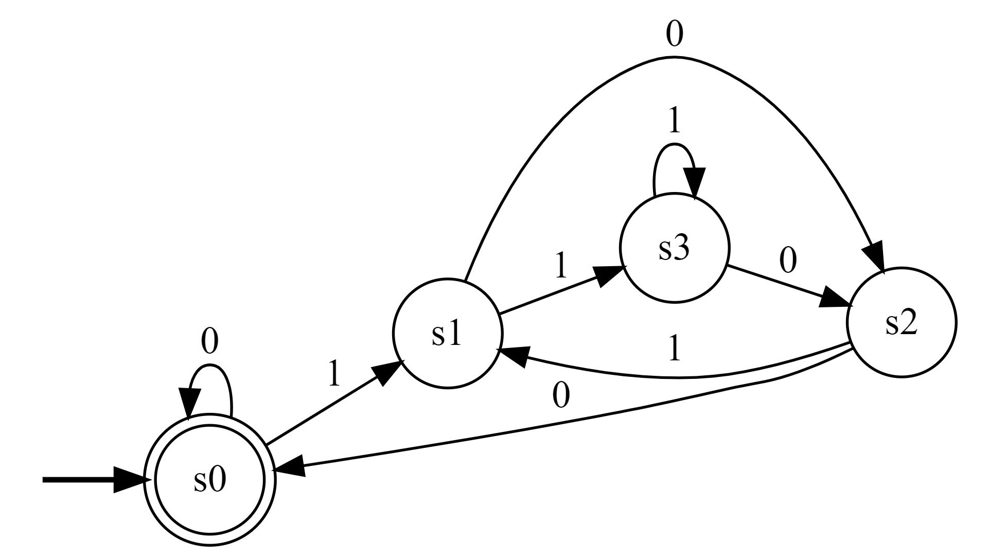
As already discussed in the previous post, any radix-b number n with nmodm∈E⊆Z can be accepted by finite automata in a digit-by-digit manner. However, the construction is not always optimal. The amount of states required is not always the amount of congruence classes. In this post we will examine when exactly the finite automata can be simplified by combining states. Reducing the amount of states will also help produce a much simpler regular expression, for example, with the Kleene construction.
In this post we will consider natural Radix-b numbers in positional number systems. The congruence class of any such arbitrary natural number can be determined by a finite automata, and thus, intuitively speaking, the language of all Radix-b numbers that satisfy some fixed properties modulo b is regular.
Typical implementation of the extended Euclidean algorithm on the internet will just iteratively calculate modulo until 0 is reached. However, sometimes you also need to calculate the linear combination coefficients for the greatest common divisor.