Using the PA=LU factorization to solve linear systems of equations for many right-hand sides efficiently

28.11.2020 in Computer Science → Linear algebra Last modified at: 18.12.2020

Linear systems of equations come up in almost any technical discipline. The PA=LU factorization method is a well-known numerical method for solving those types of systems of equations against multiple input vectors. It is also possible to preserve numerical stability by implementing some pivot strategy. In this post we will consider performance and numerical stability issues and try to cope with them by using the PA = LU factorization.

Idea behind the algorithm

Suppose we have a matrix $A$ and some set of vectors $\{b_1, \dots, b_n\}$ and we need to solve $Ax = b_i$ for all $1 \le i \le n$. Of course, we can just run the Gaussian elimination algorithm for each vector $b_i$ and compute the upper-triangular form of the matrix $A$ and then backward-substitute the vector $b_i$. However, if the set of vectors is large or the matrix itself is big, this is inefficient because we have to convert the matrix to upper-triangular form $n$ times.

While doing Gaussian elimination, all row operations are applied both to the matrix and the vector. But when we choose what operation should be applied in some step, we never consider the entries of the vector. The key idea behind the $PA = LU$ factorization algorithm is to compute the upper-triangular form of the matrix once and save all steps that have been performed so that we can perform the same steps on the current vector $b_i$ without recomputing the upper-triangular form of $A$ for backward substitution. All Gaussian elimination steps can be encoded in a matrix $L^{-1}$, such that if we multiply it by some vector $b_i$, $L^{-1}$ will apply all the operations performed while computing the upper-triangular form of $A$ to $b_i$. After that we can just do backward substitution to find $x$.

During Gaussian elimination it is possible that we are forced to swap some rows, for example if the pivot on the diagonal is zero. As we will see, it is also a good idea to swap rows not only when we are forced to do so. Anyway, in order for the algorithm to work with any matrix $A$, we need to store the permutations of the rows of $A$ in some way. For simplicity, we will store the permutation in a permutation matrix $P$ that essentially just swaps rows.

So, formally speaking, we are interested in finding such matrices $P$, $L$ and $U$, such that $PA = LU$ where $P$ is the permutation matrix, $L$ is a lower-triangular matrix and $U$ is an upper triangular matrix. We need $L$ and $U$ to be triangular matrices in order to be able to quickly solve linear systems of equations with them.

Forward and backward substitution

As already mentioned above, we need to implement forward and backward substitution in order to proceed with the $PA = LU$ factorization algorithm:

# Solves a linear system of equations Lx = b where the L matrix is lower-triangular
def forward_substitution(L, b):
    
    m = len(b)
    x = np.empty(m)
    
    for v in range(m):
        if L[v][v] == 0:
            # the value on the diagonal is zero
            x[v] = 0
            # the current variable's value is irrelevant
            continue
        # calculate v-th variable value
        value = b[v]
        # subtract linear combination of the already known variables
        # in the bottom left corner of the matrix
        for i in range(v):
            value -= L[v][i] * x[i]
        # divide by the coefficient by the v-th variable to get it's value
        value /= L[v][v]
        # store the value in the resulting vector
        x[v] = value
        
    return x

Analogously, we can implement backward substitution:

# Solves a linear system of equations Ux = b where the U matrix is upper-triangular
def backward_substitution(U, b):

    m = len(b)
    x = np.empty(m)
    
    for v in range(m - 1, -1, -1):
        if U[v][v] == 0:
            # the value on the diagonal is zero
            x[v] = 0
            continue
        # calculate v-th variable value
        value = b[v]
        # subtract linear combination of the already known variables
        # in the top right corner of the matrix
        for i in range(v + 1, m, 1):
            value -= U[v][i] * x[i]
        # divide by the coefficient before the i-th variable to get it's value
        value /= U[v][v]
        # store the value in the resulting vector
        x[v] = value
        
    return x

Solutions for non-homogeneous systems of equations are affine subspaces. If the input matrix is full-rank, i.e. doesn’t reduce the dimension of the vector space during a linear transformation, then there will be only one solution vector and the algorithms will calculate it correctly. For the sake of simplicity these algorithms just set the corresponding variables to zero if there is a zero on the diagonal, so in case the matrix is not full-rank, the algorithms will return only one vector from a set of vectors. In order to get the whole solution affine subspace it is necessary to give back a parametrized set of vectors.

PA=LU factorization

The factorization algorithm consists of the following steps:

1. Initialize $U$ with the initial matrix $A$ and let $P$ and $L$ be the identity matrices. We will transform $U$ to upper-triangular form.
2. Find some non-zero pivot element in the current column of the matrix.
3. If the found pivot element is not on the diagonal, swap the corresponding rows in the $U$ and $P$ matrices. Also, apply the swap to the part of the $L$ matrix under the main diagonal.
4. Subtract the row with the pivot on the diagonal from all rows underneath so that all element under the pivot element become zero. After $U[i][j]$ has been eliminated by subtracting $\alpha \cdot U[j]$ from row $i$, set the coefficient $L[i][j] := \alpha$ such that, in other words, $\alpha = \frac{U[i][j]}{U[j][j]}$.
5. Continue from step 2 with the next column.

The idea behind the adjustment of the $L$ matrix in step 3 is to add $\alpha \cdot \text{Pivot row}$ to the row to be eliminated and thus reverse this step. We only need to calculate the elements under the diagonal of the $L$ matrix because the row to be eliminated is always under the pivot row.

Example

Consider the following matrix: $A := \left( \begin{array}{ccc} -1 & 1 & 6 \\ -4 & -8 & 6 \\ 2 & 16 & 23 \end{array} \right)$

We can start computing the $PA = LU$ factorization by writing the initial decomposition as follows: $\left( \begin{array}{ccc} 1 & 0 & 0 \\ 0 & 1 & 0 \\ 0 & 0 & 1 \end{array} \right) \cdot A = \left( \begin{array}{ccc} 1 & 0 & 0 \\ 0 & 1 & 0 \\ 0 & 0 & 1 \end{array} \right) \cdot \left( \begin{array}{ccc} -1 & 1 & 6 \\ -4 & -8 & 6 \\ 2 & 16 & 23 \end{array} \right)$

For the first column, let’s choose the pivot $-4$ in the second row. It is not on the diagonal, so we must swap the first two rows: $\left( \begin{array}{ccc} 0 & 1 & 0 \\ 1 & 0 & 0 \\ 0 & 0 & 1 \end{array} \right) \cdot A = \left( \begin{array}{ccc} 1 & 0 & 0 \\ 0 & 1 & 0 \\ 0 & 0 & 1 \end{array} \right) \cdot \left( \begin{array}{ccc} -4 & -8 & 6 \\ -1 & 1 & 6 \\ 2 & 16 & 23 \end{array} \right)$

Now the pivot is on the diagonal and it is time to subtract $\frac{-1}{-4} = \frac{1}{4}$ of the first row from the second row and $\frac{2}{-4} = -\frac{1}{2}$ of the first row from the third row. We write these coefficients to the first column of the $L$ matrix, accordingly: $\left( \begin{array}{ccc} 0 & 1 & 0 \\ 1 & 0 & 0 \\ 0 & 0 & 1 \end{array} \right) \cdot A = \left( \begin{array}{ccc} 1 & 0 & 0 \\ \frac{1}{4} & 1 & 0 \\ -\frac{1}{2} & 0 & 1 \end{array} \right) \cdot \left( \begin{array}{ccc} -4 & -8 & 6 \\ 0 & 3 & 4.5 \\ 0 & 12 & 26 \end{array} \right)$

Now we proceed with the second column. Assume we choose $12$ as a pivot. $12$ is not on the diagonal, so we must swap the second row with the third one. This time we also need to swap the corresponding rows in the $L$ matrix: $\left( \begin{array}{ccc} 0 & 1 & 0 \\ 0 & 0 & 1 \\ 1 & 0 & 0 \end{array} \right) \cdot A = \left( \begin{array}{ccc} 1 & 0 & 0 \\ -\frac{1}{2} & 1 & 0 \\ \frac{1}{4} & 0 & 1 \end{array} \right) \cdot \left( \begin{array}{ccc} -4 & -8 & 6 \\ 0 & 12 & 26 \\ 0 & 3 & 4.5 \end{array} \right)$

We are now ready to eliminate $3$ from the third row by subtracting $\frac{3}{12} = \frac{1}{4}$ of the second row from it: $\left( \begin{array}{ccc} 0 & 1 & 0 \\ 0 & 0 & 1 \\ 1 & 0 & 0 \end{array} \right) \cdot A = \left( \begin{array}{ccc} 1 & 0 & 0 \\ -\frac{1}{2} & 1 & 0 \\ \frac{1}{4} & \frac{1}{4} & 1 \end{array} \right) \cdot \left( \begin{array}{ccc} -4 & -8 & 6 \\ 0 & 12 & 26 \\ 0 & 0 & -2 \end{array} \right)$

This is the $PA = LU$ decomposition of $A$.

Non-stable implementation

We can implement the decomposition algorithm described above in Python the following way:

# Compute the PA = LU decomposition of the matrix A
def plu(A):
    m = len(A)
    
    P = np.identity(m) # create an identity matrix of size m
    L = np.identity(m)
    
    for x in range(m):
        
        pivotRow = x
        
        if A[pivotRow][x] == 0:
            # search for a non-zero pivot
            for y in range(x + 1, m, 1):
                if A[y][x] != 0:
                    pivotRow = y
                    break
                            
        if A[pivotRow][x] == 0:
            # we didn't find any row with a non-zero leading coefficient
            # that means that the matrix has all zeroes in this column
            # so we don't need to search for pivots after all for the current column x
            continue
            
        # did we just use a pivot that is not on the diagonal?
        if pivotRow != x:
            # so we need to swap the part of the pivot row after x including x
            # with the same right part of the x row where the pivot was expected
            for i in range(x, m, 1):
                # swap the two values columnwise
                (A[x][i], A[pivotRow][i]) = (A[pivotRow][i], A[x][i])
            
            # we must save the fact that we did this swap in the permutation matrix
            # swap the pivot row with row x
            P[[x, pivotRow]] = P[[pivotRow, x]]
            
            # we also need to swap the rows in the L matrix
            # however, the relevant part of the L matrix is only the bottom-left corner
            # and before x
            for i in range(x):
                (L[x][i], L[pivotRow][i]) = (L[pivotRow][i], L[x][i])
            
        # now the pivot row is x
        # search for rows where the leading coefficient must be eliminated
        for y in range(x + 1, m, 1):
            currentValue = A[y][x]
            if currentValue == 0:
                # variable already eliminated, nothing to do
                continue
            
            pivot = A[x][x]
            assert pivot != 0 # just in case, we already made sure the pivot is not zero
            
            pivotFactor = currentValue / pivot
            
            # subtract the pivot row from the current row
            A[y][x] = 0
            for i in range(x + 1, m, 1):
                A[y][i] -= pivotFactor * A[x][i]
            
            # write the pivot factor to the L matrix
            L[y][x] = pivotFactor
        
        # the pivot must anyway be at the correct position if we found at least one
        # non-zero leading coefficient in the current column x
        assert A[x][x] != 0
        for y in range(x + 1, m, 1):
            assert A[y][x] == 0
    
    return (P, L, A)

We are now interested in solving $Ax = b$ with the computed decomposition of $A$ into $PA = LU$. It follows that $LUx = Pb$: $\begin{aligned} PA = LU &\Rightarrow PAx = LUx \\ &\Rightarrow LUx = PAx \\ &\Rightarrow LUx = Pb \end{aligned}$

We can reorder components of the vector $b$ by multiplying it with $P$ (let $z := Pb$) and then solve $Ly = z$ for $y$ using forward substitution (as $L$ is lower-triangular). Intuitively, $y := Ux$ is the vector with all the Gaussian elimination steps applied to it. After that, we can compute $x$ by solving $Ux = y$ using backward substitution (as $U$ is upper-triangular).

We can implement these steps as follows:

def plu_solve(A, b):
    (P, L, U) = plu(A)
    b = np.matmul(P, b) # multiply matrix P with vector b
    y = forward_substitution(L, b)
    x = backward_substitution(U, y)
    return x

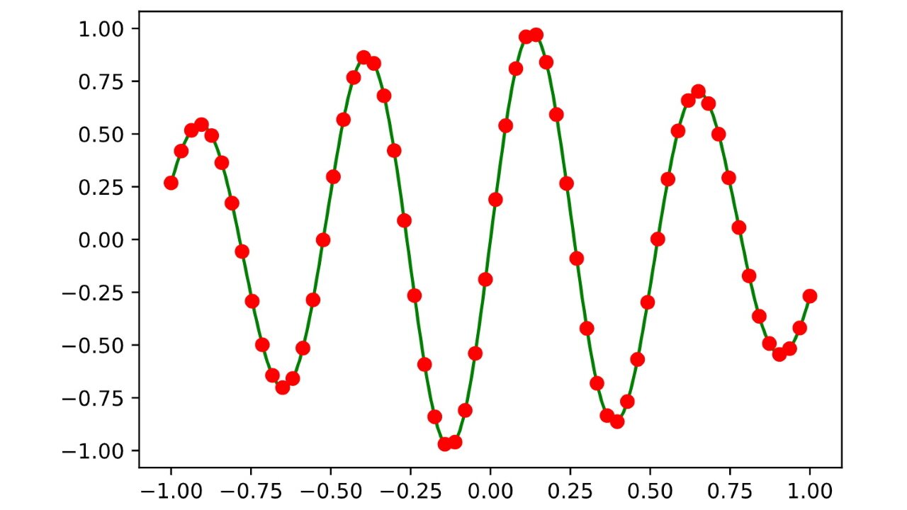
However, there it still a problem with the above implementation of plu. We can illustrate it by approximating the function $f(x) = \frac{\sin(12 \cdot x)}{x^2 + 1}$ on the interval $x \in [-1, 1]$ with the $PA = LU$ decomposition applied to a Vandermonde matrix:

As you can see, the approximation isn’t entirely right. The low-degree terms of the polynomial approximating $f(x)$ are getting lost due to rounding errors in floating point arithmetic. These low-degree terms are exactly the ones that are responsible for approximating the right part of the graph and that’s why we see rounding errors there.

Numerical stability

The issue that causes such precision problems lies in choosing the wrong pivot element. For example, consider the following matrix $A := \left( \begin{array}{cc} \varepsilon & 1 \\ 1 & 1 \end{array} \right)$

where $\varepsilon > 0$ is some very small number.

If we choose $\varepsilon$ as a pivot, then we need to subtract the second row multiplied with $\frac{1}{\varepsilon}$ to perform an elimination step. As $\varepsilon$ is very small, $\frac{1}{\varepsilon}$ is very big. So by choosing such a pivot, we not only preserve $\varepsilon$ in the matrix but also add a very large number to it, like $1 - \frac{1}{\varepsilon}$ in this case.

There are many advanced strategies to cope with this problem, but one of the most easy and effective ways to improve numerical stability is to just choose the element with the greatest absolute value as the pivot.

Thus, we can improve the implementation by adjusting the code responsible for choosing the pivot:

def palu(A):
    m = len(A)
    
    P = np.identity(m) # create an identity matrix of size m
    L = np.identity(m)
    
    for x in range(m):
        
        pivotRow = x
        
        # search for the best pivot
        for y in range(x + 1, m, 1):
            if abs(A[y][x]) > abs(A[pivotRow][x]):
                pivotRow = y
                            
        if A[pivotRow][x] == 0:
            # we didn't find any row with a non-zero leading coefficient
            # that means that the matrix has all zeroes in this column
            # so we don't need to search for pivots after all for the current column x
            continue
            
        # did we just use a pivot that is not on the diagonal?
        if pivotRow != x:
            # so we need to swap the part of the pivot row after x including x
            # with the same right part of the x row where the pivot was expected
            for i in range(x, m, 1):
                # swap the two values columnwise
                (A[x][i], A[pivotRow][i]) = (A[pivotRow][i], A[x][i])
            
            # we must save the fact that we did this swap in the permutation matrix
            # swap the pivot row with row x
            P[[x, pivotRow]] = P[[pivotRow, x]]
            
            # we also need to swap the rows in the L matrix
            # however, the relevant part of the L matrix is only the bottom-left corner
            # and before x
            for i in range(x):
                (L[x][i], L[pivotRow][i]) = (L[pivotRow][i], L[x][i])
            
        # now the pivot row is x
        # search for rows where the leading coefficient must be eliminated
        for y in range(x + 1, m, 1):
            currentValue = A[y][x]
            if currentValue == 0:
                # variable already eliminated, nothing to do
                continue
            
            pivot = A[x][x]
            assert pivot != 0 # just in case, we already made sure the pivot is not zero
            
            pivotFactor = currentValue / pivot
            
            # subtract the pivot row from the current row
            A[y][x] = 0
            for i in range(x + 1, m, 1):
                A[y][i] -= pivotFactor * A[x][i]
            
            # write the pivot factor to the L matrix
            L[y][x] = pivotFactor
        
        # the pivot must anyway be at the correct position if we found at least one
        # non-zero leading coefficient in the current column x
        assert A[x][x] != 0
        for y in range(x + 1, m, 1):
            assert A[y][x] == 0
    
    return (P, L, A)

With this implementation we get a much better approximation of $f(x)$:

Using only one matrix to store the decomposition

As $L$ is a lower-triangular matrix and $U$ is upper-triangular, we can actually create only one matrix (apart from $P$) to store the decomposition. It also allows us to simplify the way we do swap operations:

def forward_substitution(L, b):
    m = len(b)
    x = np.empty(m)
    
    for v in range(m):
        # calculate v-th variable value
        value = b[v]
        # subtract linear combination of the already known variables
        # in the bottom left corner of the matrix
        for i in range(v):
            value -= L[v][i] * x[i]
        # no need to divide by L[v][v] as it is implicitly 1, by construction
        # (this 1 is not stored in the matrix)
        # store the value in the resulting vector
        x[v] = value
        
    return x

def plu(A):
    m = len(A)
    
    P = np.identity(m)
    
    for x in range(m):
        pivotRow = x
        
        # search for the best pivot
        for y in range(x + 1, m, 1):
            if abs(A[y][x]) > abs(A[pivotRow][x]):
                pivotRow = y
                    
        if A[pivotRow][x] == 0:
            # we didn't find any row with a non-zero leading coefficient
            # that means that the matrix has all zeroes in this column
            # so we don't need to search for pivots after all for the current column x
            continue
            
        # did we just use a pivot that is not on the diagonal?
        if pivotRow != x:
            # swap the pivot row with the current row in both A and L matrices
            A[[x, pivotRow]] = A[[pivotRow, x]]
            
            # we must save the fact that we did this swap in the permutation matrix
            # swap the pivot row with row x
            P[[x, pivotRow]] = P[[pivotRow, x]]
                        
        # now the pivot row is x
        # search for rows where the leading coefficient must be eliminated
        for y in range(x + 1, m, 1):
            currentValue = A[y][x]
            if currentValue == 0:
                # variable already eliminated, nothing to do
                continue
            
            pivot = A[x][x]
            assert pivot != 0 # just in case, we already made sure the pivot is not zero
            
            pivotFactor = currentValue / pivot
            
            # subtract the pivot row from the current row
            for i in range(x + 1, m, 1):
                A[y][i] -= pivotFactor * A[x][i]
            
            # write the pivot factor to the L matrix
            A[y][x] = pivotFactor
    
    return (P, A)

def plu_solve(P, LU, b):
    b = np.matmul(P, b)
    y = forward_substitution(LU, b)
    x = backward_substitution(LU, y)
    return x

It is possible to further optimize the algorithms by removing the permutation matrix $P$ and replacing it with a simple array that permutes it’s indices (or some other permutation datastructure).

As already mentioned in the beginning of the post, the key advantage of the $PA = LU$ decomposition is that it allows us to solve linear systems of equations for many input vectors from $B := \{b_1, \dots, b_n\}$ by doing Gaussian elimination only once

(P, LU) = plu(A)
for b in B:
    solution = plu_solve(P, LU, b)

instead of doing full Gaussian elimination $n$ times.

Let $m$ be the size of the vector and $A$ be an $m \times m$ matrix. Then the complexity of computing the $PA = LU$ factorization is $O(m^3)$. If we optimize the permutation matrix so that permuting elements takes time in $O(m^2)$, then the solving algorithm’s complexity is $O(m^2)$.

Therefore, the overall complexity of the algorithm that takes $A$ and a set of $n$ vectors $B$ and solves $Ax = b$ for every $b \in B$ (as shown in the code snippet above) is $O(m^3 + n \cdot m^2)$, which is better than $O(n \cdot m^3)$ if we apply Gaussian elimination $n$ times.