Kadane's algorithm and the idea behind it

19.09.2020 in Computer Science Last modified at: 22.10.2020

People often refer to Kadane’s algorithm only in the context of the maximum subarray problem. However, the idea behind this algorithm allows one to use it for solving a variety of problems that have something to do with finding a continuous subarray with a given property. The algorithm can also be used in 2d or multidimensional arrays but in this post we will only consider regular one-dimensional arrays.

Motivation & idea

If we are searching for a subarray with some property, the easiest solution would be to try all possible intervals. A naive algorithm can do that in $O(n^3)$ time, but we can improve that by computing solutions for intervals of increasing length and reusing already computed solutions (aka dynamic programming). In this case the complexity of the algorithm is $O(n^2)$. Of course, this will work not for all problems. It will work, for example, for the computation of any binary associative operation for all intervals in the array. Another example for such an algorithm would be finding all palindromes in a given string:

• Mark all letters as palindromes of length 1
• Mark all adjacent equal letters as palindromes of length 2
• For every fixed length $k$, starting with $k = 3$ traverse all substrings of length $k$ in the string and mark the current substring as a palindrome if the letters at the start and at the end match and if the middle part is a palindrome.

$O(n^2)$ is the optimal worst-case complexity if the problem cannot be solved without traversing the entire search space. For example, this is the case for the problem of computing all palindromes of a given string (a worst-case example is $a^n \in \Sigma^*$ where the amount of palindromes is $\sum_{i=1}^{n}i =\frac{n \cdot (n + 1)}{2} \in \Omega(n^2)$).

The key question is: How can we traverse only some subset of the search space and still benefit from dynamic programming?

Well, we can identify a problem with only one side of the interval in the array. We will choose the right side of the interval because that is what is commonly used in real algorithms. That way it is possible to construct a linear time algorithm the following way:

• Create a recursive function $f(k)$ that computes the trivial solution if $k = 1$ and computes the new solution based on the already computed result, e.g. $f(k-1)$.
• Find the best solution among $\{f(k) : 0 \le k < n\}$.

Both parts take linear ($O(n)$) time if we cache and reuse the result of $f(k)$ or if we use dynamic programming which is better most of the times.

Maximum sum subarray

A good example for a construction of such an algorithm is the maximum sum subarray problem - given an array $A$ of integers the algorithm should find such indices $a,b \in \{1, \dots, n-1\}$ with $a \le b$ such that $\sum_{i=a}^b {A[i]}$ is maximal.

We can define the problem only in terms of the right border $k$ - “what is the maximum subarray ending at $k$”?

Clearly, the maximum subarray of the whole array is the maximum of subarrays ending at $k$ for all $0 \le k < n$. Also, the maximum sum subarray ending at k is either $A[k]$ itself or the maximum sum subarray ending at $k - 1$ combined with $A[k]$. So we can now write the algorithm formally with pseudocode:

maxSumSubarrayEndingAt(A, k) {
    if (k == 0) {
        return (A[0], 1);
    }
    (sum, left) = maxSumSubarrayEndingAt(k - 1);
    if (sum >= 0) { /* sum + A[k] >= A[k] */
        /* the max subarray (ending at k) is the previous subarray together with this element */
        return (sum + A[k], left);
    }
    else {
        /* the max subarray (ending at k) is the current element */
        return (A[k], k);
    }
}

And the maximum subarray sum and indices can be computed with a simple maximim-search algorithm:

maxSumSubarray(A) {
    n = size(A);
    maxSum = A[0];
    maxLeft = 0;
    maxRight = 0;
    for (r = 1; r < n; r++) {
        (s, l) = maxSumSubarrayEndingAt(A, r);
        if (s > maxSum) {
            maxSum = s;
            maxLeft = l;
            maxRight = r;
        }
    }
    return (maxSum, maxLeft, maxRight);
}

This intermediate pseudocode solution doesn’t cache maxSumSubarrayEndingAt results and is therefore inefficient “as-is”. But we can remove recursion and rewrite the same solution with dynamic programming (Java):

public static void maxSumSubarray(int[] a) {
    int maxSum = a[0];
    int maxLeft = 0;
    int maxRight = 0;

    int currentSum = a[0];
    int currentLeft = 0;

    for (int r = 1; r < a.length; r++) {

        if (currentSum >= 0) {
            currentSum += a[r];
        }
        else {
            currentSum = a[r];
            currentLeft = r;
        }

        if (currentSum > maxSum) {
            maxSum = currentSum;
            maxLeft = currentLeft;
            maxRight = r;
        }
    }

    // the sum between A[maxLeft] and A[maxRight] (inclusive) is equal maxSum and maximal
    System.out.printf("Max sum: %5d Indices from %5d to %5d.\n", maxSum, maxLeft, maxRight);
}

This is the efficient $\Theta(n)$ time and $\Theta(1)$ space solution that uses the idea of Kadane’s algorithm to compute the maximum sum subarray.

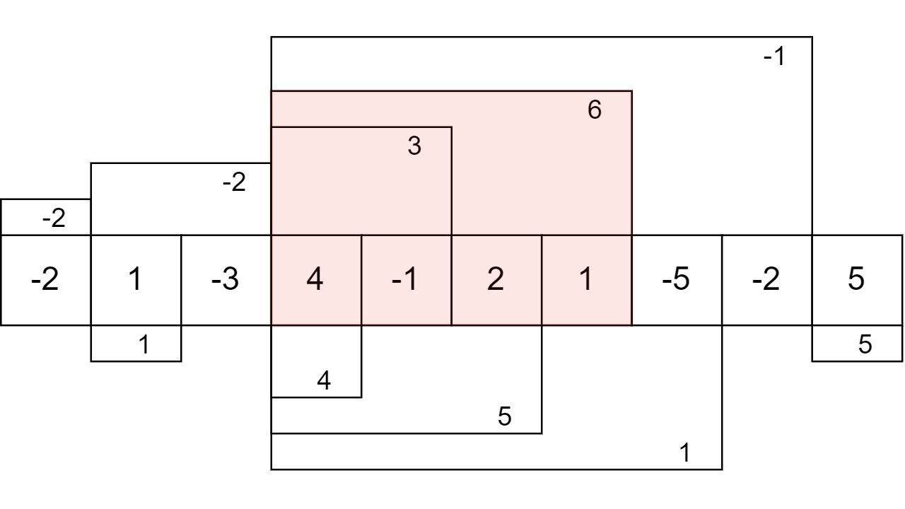
Example

Consider the array {-2, 1, -3, 4, -1, 2, 1, -5, -2, 5}. By running the algorithm we get the following maximum subarrays ending at a specific index:

The maximum subarray is marked red.

Other problems that can be solved analogously

• Smallest sum subarray problem
• Largest product subarray problem
• Smallest product subarray problem
• Maximum circular sum