Visualizing 3D linear transformations and Gaussian elimination with Python and Manim
Matrices are omnipresent in linear algebra. Columns of a matrix describe where the corresponding basis vectors land relative to the initial basis. All transformed vectors are linear combinations of transformed basis vectors which are the columns of the matrix, this is also called linearity. Algorithms that operate on matrices essentially just alter the way vectors get transformed, preserving some properties. Unfortunately, many algorithms are typically presented to students in a numerical fashion, without describing the whole graphical meaning. In this post we will first visualize simple linear transformations and then we will visualize Gaussian Elimination (with row swaps) steps as a sequence of linear transformations. To do this, we will use Python together with a popular Open-Source library manim.
Visualizing 3D transformations
In manim, there is a special ApplyMatrix animation that allows us to natively apply a matrix to every 3D vertex of the object.
from manimlib.imports import *

class LinearTransformation3D(ThreeDScene):

    CONFIG = {
        "x_axis_label": "$x$",
        "y_axis_label": "$y$",
        "basis_i_color": GREEN,
        "basis_j_color": RED,
        "basis_k_color": GOLD
    }

    def create_matrix(self, np_matrix):

        m = Matrix(np_matrix)

        m.scale(0.5)
        m.set_column_colors(self.basis_i_color, self.basis_j_color, self.basis_k_color)

        m.to_corner(UP + LEFT)

        return m

    def construct(self):

        M = np.array([
            [2, 2, -1],
            [-2, 1, 2],
            [3, 1, -0]
        ])

        axes = ThreeDAxes()
        axes.set_color(GRAY)
        axes.add(axes.get_axis_labels())

        self.set_camera_orientation(phi=75 * DEGREES, theta=-45 * DEGREES)

        # basis vectors i,j,k
        basis_vector_helper = TextMobject("$i$", ",", "$j$", ",", "$k$")
        basis_vector_helper[0].set_color(self.basis_i_color)
        basis_vector_helper[2].set_color(self.basis_j_color)
        basis_vector_helper[4].set_color(self.basis_k_color)

        basis_vector_helper.to_corner(UP + RIGHT)

        self.add_fixed_in_frame_mobjects(basis_vector_helper)

        # matrix
        matrix = self.create_matrix(M)

        self.add_fixed_in_frame_mobjects(matrix)

        # axes & camera
        self.add(axes)

        self.begin_ambient_camera_rotation(rate=0.2)

        cube = Cube(side_length=1, fill_color=BLUE, stroke_width=2, fill_opacity=0.1)
        cube.set_stroke(BLUE_E)

        i_vec = Vector(np.array([1, 0, 0]), color=self.basis_i_color)
        j_vec = Vector(np.array([0, 1, 0]), color=self.basis_j_color)
        k_vec = Vector(np.array([0, 0, 1]), color=self.basis_k_color)

        i_vec_new = Vector(M @ np.array([1, 0, 0]), color=self.basis_i_color)
        j_vec_new = Vector(M @ np.array([0, 1, 0]), color=self.basis_j_color)
        k_vec_new = Vector(M @ np.array([0, 0, 1]), color=self.basis_k_color)

        self.play(
            ShowCreation(cube),
            GrowArrow(i_vec),
            GrowArrow(j_vec),
            GrowArrow(k_vec),
            Write(basis_vector_helper)
        )

        self.wait()

        matrix_anim = ApplyMatrix(M, cube)

        self.play(
            matrix_anim,
            Transform(i_vec, i_vec_new, rate_func=matrix_anim.get_rate_func(),
                      run_time=matrix_anim.get_run_time()),
            Transform(j_vec, j_vec_new, rate_func=matrix_anim.get_rate_func(),
                      run_time=matrix_anim.get_run_time()),
            Transform(k_vec, k_vec_new, rate_func=matrix_anim.get_rate_func(),
                      run_time=matrix_anim.get_run_time())
        )

        self.wait()

        self.wait(7)
With this implementation we can visualize, for example, the following matrix presented in the video (top left corner):
We can also visualize what it means for 2 columns to be linear dependent — the cube gets squashed into a plane:
Visualizing Gaussian elimination
In the previous post we implemented an advanced version of the Gaussian elimination algorithm with pivoting (the decomposition). We can analogously implement the pure Gaussian Elimination algorithm with pivoting the following way:
def gauss(a):
    m = a.shape[0]

    for x in range(m):
        pivotRow = x

        # search for the best pivot
        for y in range(x + 1, m, 1):
            if abs(a[y][x]) > abs(a[pivotRow][x]):
                pivotRow = y

        if a[pivotRow][x] == 0:
            # we didn't find any row with a non-zero leading coefficient
            # that means that the matrix has all zeroes in this column
            # so we don't need to search for pivots after all for the current column x
            continue

        # did we just use a pivot that is not on the diagonal?
        if pivotRow != x:
            # swap the pivot row with the current row in both A and L matrices
            a[[x, pivotRow]] = a[[pivotRow, x]]
            yield a

        # now the pivot row is x
        # search for rows where the leading coefficient must be eliminated
        for y in range(x + 1, m, 1):
            currentValue = a[y][x]
            if currentValue == 0:
                # variable already eliminated, nothing to do
                continue

            pivot = a[x][x]
            assert pivot != 0  # just in case, we already made sure the pivot is not zero

            pivotFactor = currentValue / pivot

            # subtract the pivot row from the current row

            a[y][x] = 0

            for i in range(x + 1, m, 1):
                a[y][i] -= pivotFactor * a[x][i]

            yield a
Notice that after every matrix operation we want to visualize I’ve added a yield statement. Generators in Python are perfect for visualizing algorithms, because they allow us to save the current state, yield the value and then continue the execution when the caller handled the received value. In this case, we yield every version of the matrix as the algorithm runs.
Now we can adjust and extend the code used to render linear transformations to do this for every step of the gaussian elimination:
class Gauss3D(ThreeDScene):
CONFIG = {
"x_axis_label": "$x$",
"y_axis_label": "$y$",
"basis_i_color": GREEN,
"basis_j_color": RED,
"basis_k_color": GOLD
}
def create_matrix(self, np_matrix):
m = Matrix(np_matrix)
m.scale(0.5)
m.set_column_colors(self.basis_i_color, self.basis_j_color, self.basis_k_color)
m.to_corner(UP + LEFT)
return m
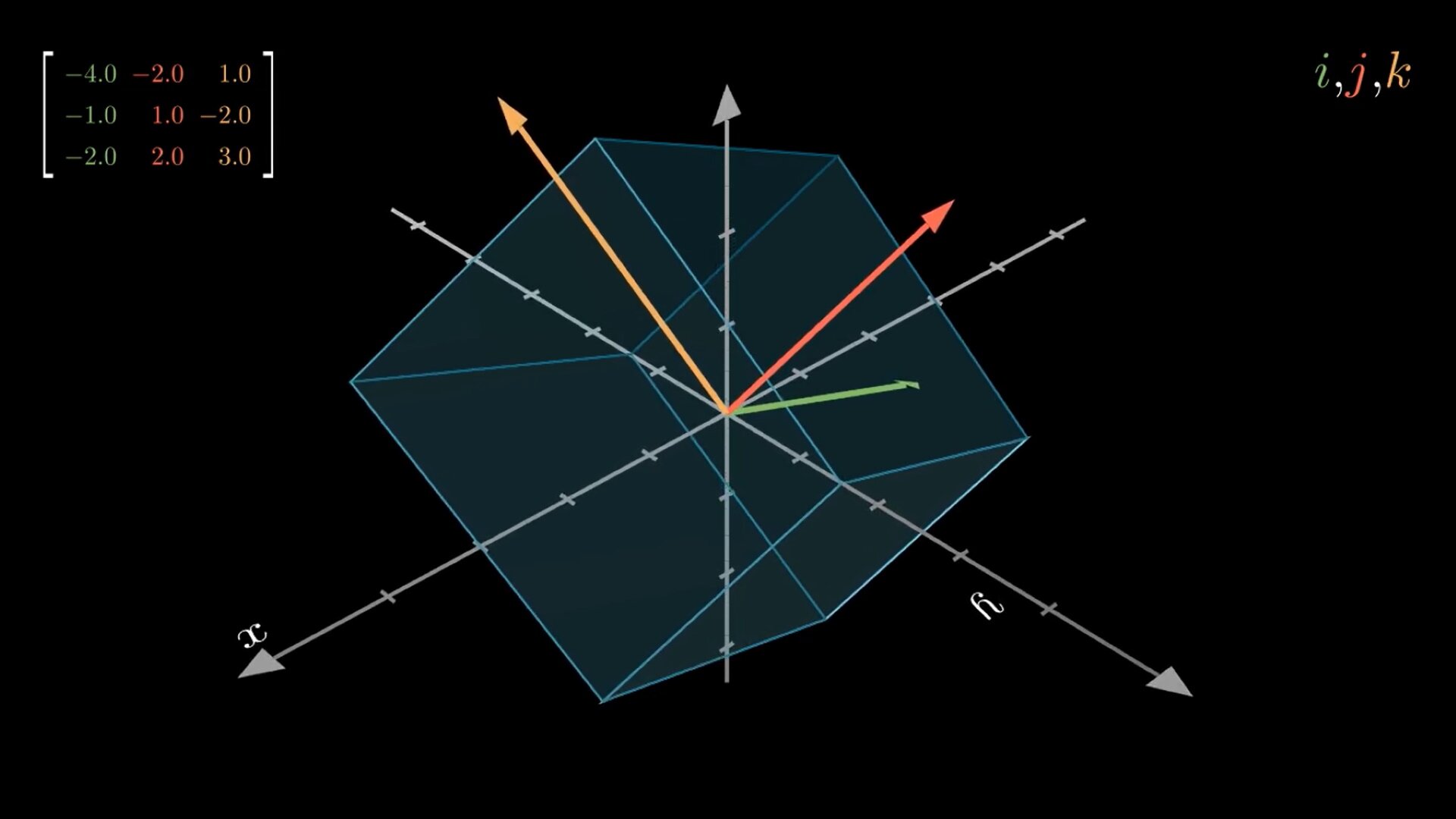
def construct(self):
M = np.array([
[-1.0, 1.0, -2.0],
[-4.0, -2.0, 1.0],
[-2.0, 2.0, 3.0]
])
# axes
axes = ThreeDAxes()
axes.set_color(GRAY)
axes.add(axes.get_axis_labels())
self.set_camera_orientation(phi=55 * DEGREES, theta=-45 * DEGREES)
# basis vectors i,j,k
basis_vector_helper = TextMobject("$i$", ",", "$j$", ",", "$k$")
basis_vector_helper[0].set_color(self.basis_i_color)
basis_vector_helper[2].set_color(self.basis_j_color)
basis_vector_helper[4].set_color(self.basis_k_color)
basis_vector_helper.to_corner(UP + RIGHT)
self.add_fixed_in_frame_mobjects(basis_vector_helper)
# matrix
matrix = self.create_matrix(M)
self.add_fixed_in_frame_mobjects(matrix)
# axes & camera
self.add(axes)
self.begin_ambient_camera_rotation(rate=0.15)
cube = Cube(side_length=1, fill_color=BLUE, stroke_width=2, fill_opacity=0.1)
cube.set_stroke(BLUE_E) # cube.set_stroke(TEAL_E)
i_vec = Vector(np.array([1, 0, 0]), color=self.basis_i_color)
j_vec = Vector(np.array([0, 1, 0]), color=self.basis_j_color)
k_vec = Vector(np.array([0, 0, 1]), color=self.basis_k_color)
i_vec_new = Vector(M @ np.array([1, 0, 0]), color=self.basis_i_color)
j_vec_new = Vector(M @ np.array([0, 1, 0]), color=self.basis_j_color)
k_vec_new = Vector(M @ np.array([0, 0, 1]), color=self.basis_k_color)
self.play(
ShowCreation(cube),
GrowArrow(i_vec),
GrowArrow(j_vec),
GrowArrow(k_vec),
Write(basis_vector_helper)
)
self.wait()
matrix_anim = ApplyMatrix(M, cube)
self.play(
matrix_anim,
ReplacementTransform(i_vec, i_vec_new, rate_func=matrix_anim.get_rate_func(),
run_time=matrix_anim.get_run_time()),
ReplacementTransform(j_vec, j_vec_new, rate_func=matrix_anim.get_rate_func(),
run_time=matrix_anim.get_run_time()),
ReplacementTransform(k_vec, k_vec_new, rate_func=matrix_anim.get_rate_func(),
run_time=matrix_anim.get_run_time())
)
self.wait()
i_vec, j_vec, k_vec = i_vec_new, j_vec_new, k_vec_new
self.wait(2)
for a in gauss(M):
a_rounded = np.round(a.copy(), 2)
self.remove(matrix)
matrix = self.create_matrix(a_rounded)
self.add_fixed_in_frame_mobjects(matrix)
# transformed cube
new_cube = Cube(side_length=1, fill_color=BLUE, stroke_width=2, fill_opacity=0.1)
new_cube.set_stroke(BLUE_E)
new_cube.apply_matrix(a)
# vectors
i_vec_new = Vector(a @ np.array([1, 0, 0]), color=self.basis_i_color)
j_vec_new = Vector(a @ np.array([0, 1, 0]), color=self.basis_j_color)
k_vec_new = Vector(a @ np.array([0, 0, 1]), color=self.basis_k_color)
# prepare and run animation
cube_anim = ReplacementTransform(cube, new_cube)
self.play(
cube_anim,
ReplacementTransform(i_vec, i_vec_new, rate_func=cube_anim.get_rate_func(),
run_time=cube_anim.get_run_time()),
ReplacementTransform(j_vec, j_vec_new, rate_func=cube_anim.get_rate_func(),
run_time=cube_anim.get_run_time()),
ReplacementTransform(k_vec, k_vec_new, rate_func=cube_anim.get_rate_func(),
run_time=cube_anim.get_run_time())
)
self.wait()
cube = new_cube
i_vec, j_vec, k_vec = i_vec_new, j_vec_new, k_vec_new
self.wait(1)
self.wait(1)
We can now see graphically how the column vectors get aligned as we bring the matrix to upper triangular form: