Compressing images with singular value decomposition (SVD)
The singular matrix decomposition plays a major role in linear algebra and has a lot of applications, including lossy image compression. In this post we will discuss it in the context of the mentioned image compression with the focus on the intuition behind the algorithm, without going deep into the theory.
SVD and the idea behind it
Any matrix describes some linear transformation from to by specifying in it’s columns where the basis vectors should land relative to the initial basis. Basically, linear transformations are able to stretch, rotate and flip space and, of course, do any combination of these actions at once. So we might be interested in creating some kind of normal form for linear transformations consisting of only geometrically simple operations, so that we are able to convert any linear transformation to this normal form. This is the key idea behind SVD — it is a normal form that consists of 2 rotations and 1 scaling.
Formally, any matrix can be written as
where:
- is an orthogonal matrix that rotates space, column vectors of this matrix are often referred to as left singular vectors.
- is a diagonal matrix (all elements that are not on the diagonal are zero, diagonal elements are called singular values), which scales space.
- is an orthogonal matrix, which only rotates space. Row vectors of are also known as right singular vectors.
- Singular values (on the diagonal) of are sorted in descending order and are different. We will denote them with where is the amount of non-zero entries on the diagonal (it also follows, that ).
So, any linear transformation can be decomposed in a rotation , followed by some scaling by , followed by another rotation .
Visualizing SVD
Consider the following simple shear matrix:
We can use the Open Source manim python library to visualize as well as its decomposition :
# file: "svd_2d.py"
from manimlib.imports import *


class SVD_2D(LinearTransformationScene):
    CONFIG = {
        "include_background_plane": True,
        "include_foreground_plane": True,
        "foreground_plane_kwargs": {
            "x_radius": FRAME_WIDTH,
            "y_radius": FRAME_HEIGHT,
            "secondary_line_ratio": 0
        },
        "background_plane_kwargs": {
            "color": GREY,
            "secondary_color": DARK_GREY,
            "axes_color": GREY,
            "stroke_width": 2,
        },
        "show_coordinates": True,
        "show_basis_vectors": True,
        "basis_vector_stroke_width": 6,
        "i_hat_color": X_COLOR,
        "j_hat_color": Y_COLOR,
        "leave_ghost_vectors": False
    }

    def construct(self):

        circle = Circle()
        circle.move_to(RIGHT + UP)

        self.add_transformable_mobject(circle)

        text_applying = TextMobject("Applying $ A $ (overall transformation)")
        text_applying.to_edge(UP + LEFT)

        text_applying_inverse = TextMobject("Applying $ A^{-1} $ (resetting)")
        text_applying_inverse.to_edge(UP + LEFT)

        text_applying_vt = TextMobject(r"Applying $ V^\top $ (rotating)")
        text_applying_vt.to_edge(UP + LEFT)

        text_applying_s = TextMobject(r"Applying $ \Sigma $ (stretching)")
        text_applying_s.to_edge(UP + LEFT)

        text_applying_u = TextMobject("Applying $ U $ (rotating)")
        text_applying_u.to_edge(UP + LEFT)

        A = np.array([
            [1, 1],
            [0, 1]
        ])

        self.play(Write(text_applying), run_time=0.5)
        self.apply_matrix(A)

        self.wait()
        self.wait(0.5)

        self.leave_ghost_vectors = True

        self.play(ReplacementTransform(text_applying, text_applying_inverse), run_time=0.5)
        self.apply_inverse(A)

        self.wait()
        self.wait(0.5)

        self.leave_ghost_vectors = False

        U, S, VT = np.linalg.svd(A)

        self.play(ReplacementTransform(text_applying_inverse, text_applying_vt), run_time=0.5)
        self.apply_matrix(VT)

        self.wait()
        self.wait(0.5)

        self.play(ReplacementTransform(text_applying_vt, text_applying_s), run_time=0.5)
        self.apply_matrix(np.diag(S))

        self.wait()
        self.wait(0.5)

        self.play(ReplacementTransform(text_applying_s, text_applying_u), run_time=0.5)
        self.apply_matrix(U)

        self.wait()
        self.wait(0.5)
In order to compute the SVD decomposition, I used the np.linalg.svd function which returns the tuple with the , and matrices as expected. However, for efficiency reasons numpy returnes as a vector (It doesn’t make sense to store zeroes that are off the diagonal). So that’s why I later on use np.diag to convert a vector to a matrix with the vector on the diagonal.
By running manim with the command manim svd_2d.py SVD_2D -m, we get:
As you can see, the geometric properties of the matrices in the decompositions as described above hold ( and rotate space, only stretches it).
Compressing images with SVD
Any image can be represented as a matrix of pixels, where each pixel (typically) consists of 3 bytes — for the red, green and blue components of the color, respectively. So, if we want to efficiently store the image, we need to somehow efficiently encode 3 matrices , and for each color component, respectively.
Let’s focus on compressing just one matrix . As stated above, applying the SVD decomposition gives us:
We can re-write this decomposition in a slightly different way:
With this notation, we can think of SVD from a slightly different perspective — SVD allows us to take an arbitrary matrix and write it down as a sum of rank-1 matrices.
If we take a random matrix , it is very unlikely that it will not be full-rank. So for a random image of width and height , the matrix will almost certainly have rank . We can approximate with the first summands:
This approximation is good, because — first singular values contribute more than the following. By the way, the Eckhart-Young theorem states that such an approximation is indeed the best possible one, so, restricted to the model in which we approximate a matrix with a sum of rank-1 matrices, we get the best possible compression algorithm.
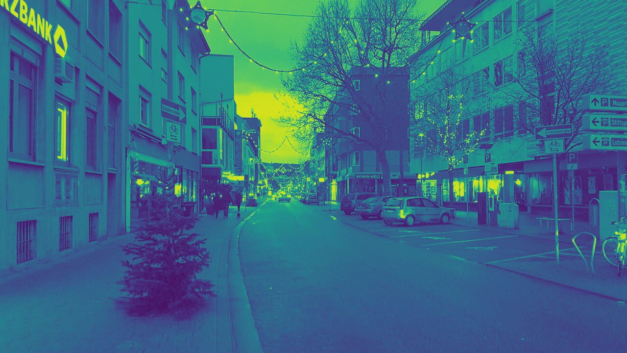
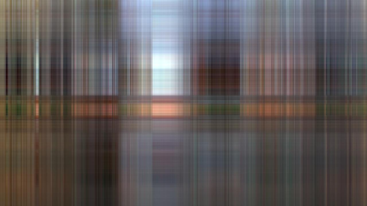
With this approximation idea we are now ready to implement image compression. Let’s start with some image — for example with this photo I recently took in Kaiserslautern, Germany:
If the image is saved as img.jpg, we can read it with:
import numpy as np

import matplotlib
import matplotlib.image as image

A = image.imread("img.jpg")
We can extract the 3 color component matrices as briefly mentioned above as follows:
R = A[:,:,0] / 0xff
G = A[:,:,1] / 0xff
B = A[:,:,2] / 0xff
Now, we compute the SVD decomposition:
R_U, R_S, R_VT = np.linalg.svd(R)
G_U, G_S, G_VT = np.linalg.svd(G)
B_U, B_S, B_VT = np.linalg.svd(B)
Now we need to determine , with which we will approximate the 3 matrices. There are different ways of doing it — I will just calculate the maximum rank of the compressed image, divided by the maximum possible rank of the initial matrix (which is the width of the image) and call this ratio the relative rank.
relative_rank = 0.2
max_rank = int(relative_rank * min(R.shape[0], R.shape[1]))
print("max rank = %d" % max_rank)  # 144
Now, we can implement a function that will only use the first columns of the matrix and the first rows of the matrix, as well as . By doing this, we essentially emulate what a decompressing algorithm would do.
def read_as_compressed(U, S, VT, k):
    A = np.zeros((U.shape[0], VT.shape[1]))
    for i in range(k):
        U_i = U[:,[i]]
        VT_i = np.array([VT[i]])
        A += S[i] * (U_i @ VT_i)
    return A
Actually, it is easier and more efficient to perform the same operation with a lower-rank matrix multiplication.
def read_as_compressed(U, S, VT, k):
    return (U[:,:k] @ np.diag(S[:k])) @ VT[:k]
So we can compute the color matrices of the approximated image with:
R_compressed = read_as_compressed(R_U, R_S, R_VT, max_rank)
G_compressed = read_as_compressed(G_U, G_S, G_VT, max_rank)
B_compressed = read_as_compressed(B_U, B_S, B_VT, max_rank)

compressed_float = np.dstack((R_compressed, G_compressed, B_compressed))
compressed = (np.minimum(compressed_float, 1.0) * 0xff).astype(np.uint8)
With matplotlib, we can also easily plot both the original as well as the compressed image by simply calling:
import matplotlib.pyplot as plt

plt.figure(figsize = (16, 9))
plt.imshow(A)

plt.figure(figsize = (16, 9))
plt.imshow(compressed)

image.imsave("compressed.png", compressed)
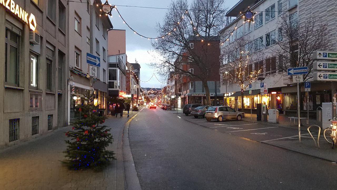
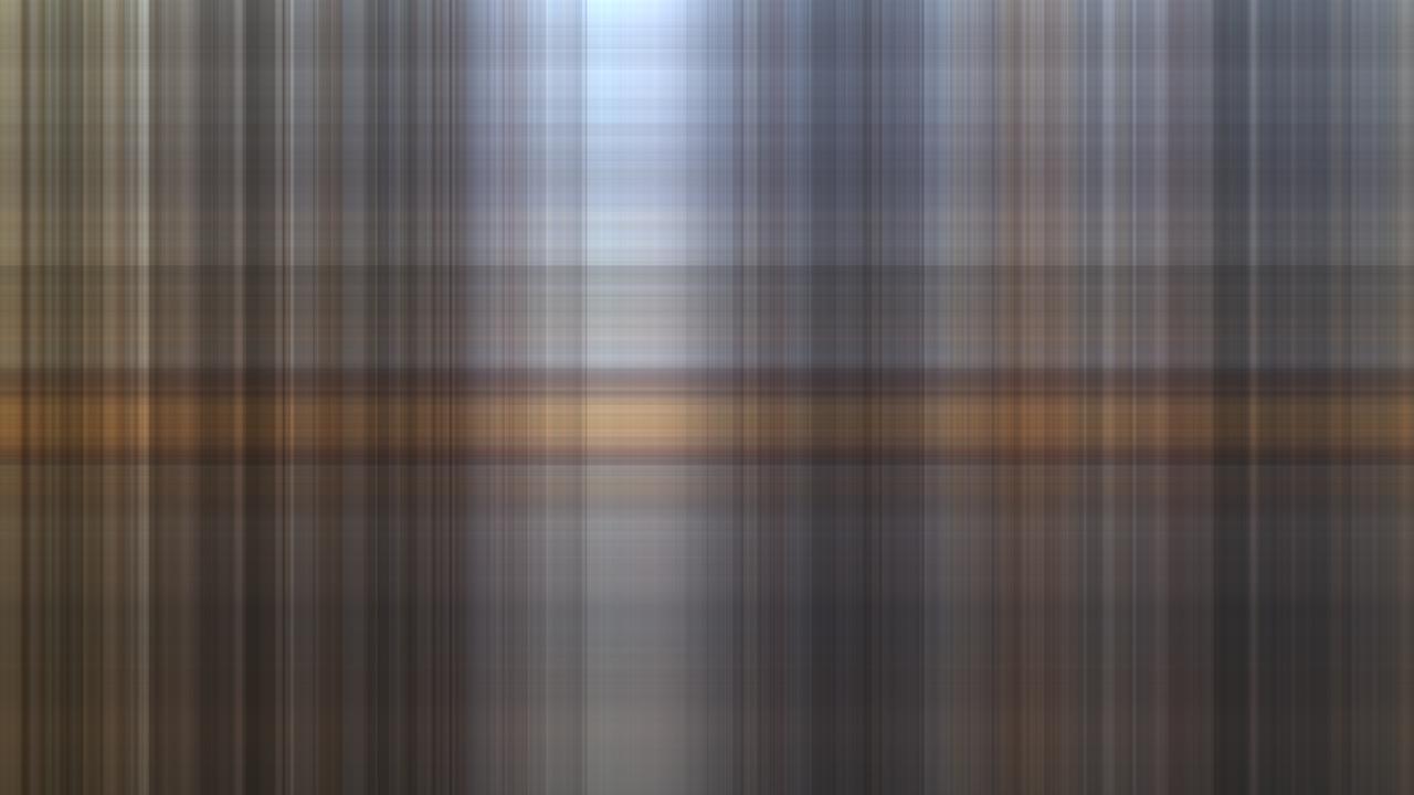
By approximating the image with a matrix of maximum rank equal to of the maximum rank of the original image, we get:

We can also run the algorithm for other relative rank values:
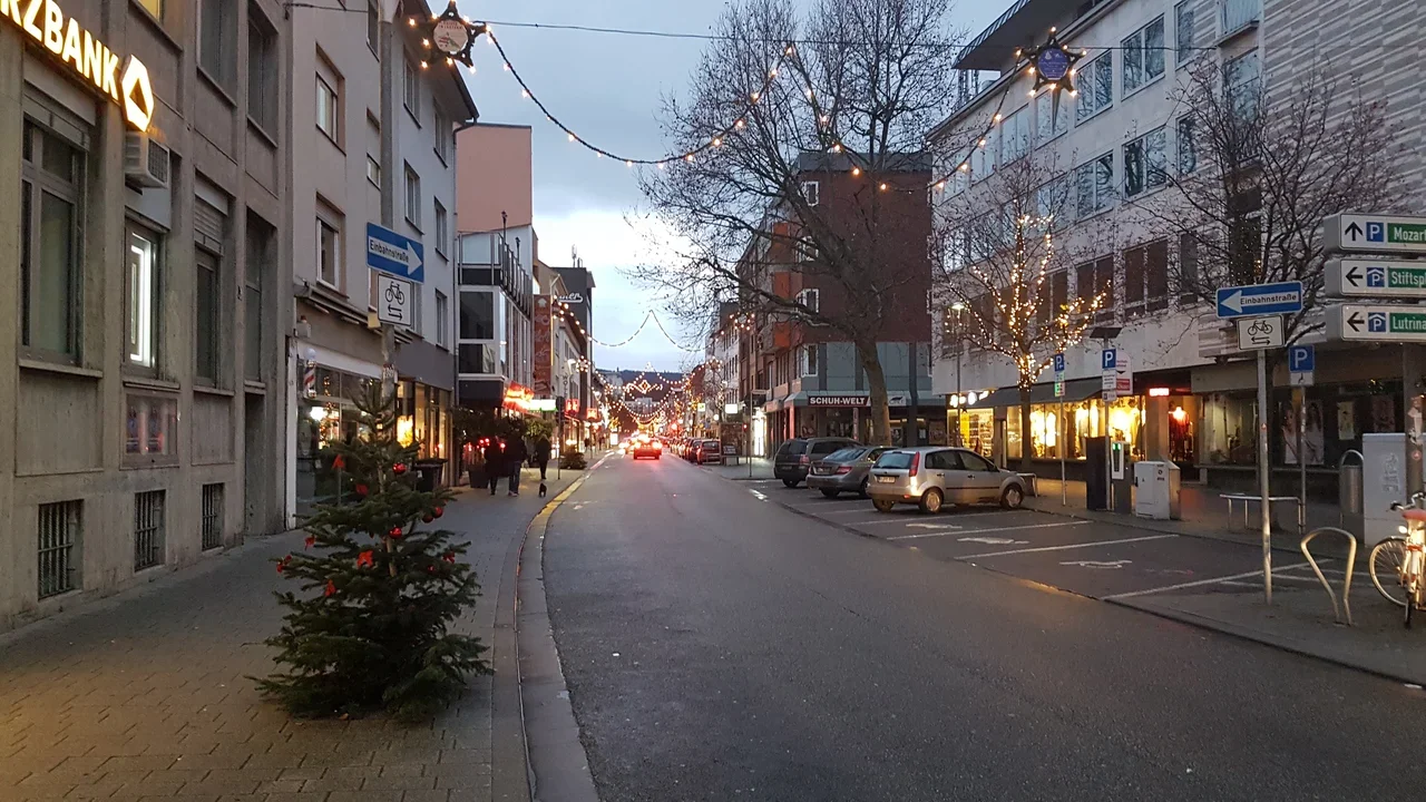
Relative rank = , Rank: and we get the original image:
Relative rank = , Rank: :

Relative rank = , Rank: :

Relative rank = , Rank: :

Relative rank = , Rank: :

Relative rank = , Rank: :

Relative rank = , Rank: :
Relative rank = , Rank: :

Relative rank = , Rank: :
Relative rank = , Rank: :

Relative rank = , Rank: :

Relative rank = , Rank: :

Relative rank = , Rank: :
Relative rank = , Rank: :
Relative rank = , Rank: :
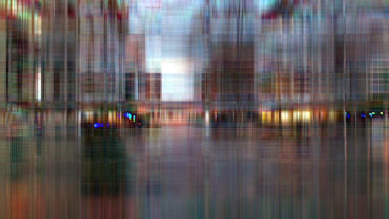
Relative rank = , Rank: :
In this case we don’t approximate at all and thus get the zero-matrix which means all pixels are black:
