Visualization and detailed description of the interactive protocol for TQBF yielding IP = PSPACE

03.04.2022 in Computer Science → Complexity theory, Logic Last modified at: 09.04.2022

In complexity theory, it is well known that IP = PSPACE. In this post I would like to go over the private coin interactive protocol for TQBF typically used to prove that PSPACE is contained in IP and, in that context, present my detailed visualization of the entire protocol together with the Open Source tool I developed to run the protocol and render the animations. I would also like to note that when I was first studying the proof protocol for TQBF, I was a bit frustrated by the fact that most texts lack a precise and detailed description of some subtleties in the proof — this is what also motivated me to try my best to fill in the relevant but missing details in this post.

Shamir’s Theorem

In 1990, Adi Shamir proved that $\operatorname{IP} = \operatorname{PSPACE}$. I find this result quite surprising, because it shows that just allowing the verifier to toss coins increases the computational power of polynomially long lasting interactive proof systems drastically, namely from $\operatorname{dIP} = \operatorname{NP}$ to $\operatorname{PSPACE}$. It is not hard to see why $\operatorname{IP} \subseteq \operatorname{PSPACE}$ — this is the case because we can try running the interactive proof system for all possible random bits the verifier may use and messages the prover could potentially send. After that, it is possible to check whether we were able to find a way to convince the verifier for most possibilities of choosing random bits. More precisely, a $\operatorname{PSPACE}$ decider for $L \in \operatorname{IP}$ can be constructed as follows (pseudocode):

c = 0
threshold = ceil(2/3 * (total number of different ways the verifier can toss coins))
for all possible verifier's random bits {
    for all possible message sequences the prover may send during the communication {
        Run the verifier using the current message sequence and random bits;
        if verifier accepted {
            c++;
            break;
        }
    }
}
if c >= threshold {
    accept;
} else {
    reject;
}

So the main challenge of showing $\operatorname{IP} = \operatorname{PSPACE}$ is actually showing that $\operatorname{PSPACE} \subseteq \operatorname{IP}$. Since $\operatorname{IP}$ is closed under polynomial time Karp reductions and $\operatorname{TQBF}$ is $\operatorname{PSPACE}$-complete, it suffices to show that $\operatorname{TQBF} \in \operatorname{IP}$. There are multiple ways of proving it — I will generally follow Shamir’s approach and use a trick called linearization, which was introduced by Shen in this paper.

Arithmetization

The main tool used in the proof is arithmetization, that is, the representation of QBF sentences using polynomials. Assuming without loss of generality that the given quantified boolean formula $\varphi = \mathcal{Q}_1 x_1 \dots \mathcal{Q}_n x_n \varphi'(x_1, \dots, x_n), \quad\mathcal{Q}_i \in \{\exists, \forall\}$

is in prenex normal form with matrix $\varphi'$ in CNF, we can obtain a polynomial $P_{\varphi}$ by essentially thinking of disjunctions as negated conjunctions and by simulating conjunctions with multiplication. Formally, if $x_i$ is an arbitrary variable, $l_{i_j}$ is an arbitrary literal and $C_i$ is an arbitrary clause appearing in $\varphi' = C_1 \wedge \dots C_m$, then we can define the arithmetizing polynomial $P_{\varphi} := P(\varphi')$ recursively as follows: $\begin{aligned} P(x_i) &:= 1 - x_i \\ P(\overline{x_i}) &:= x_i \\ P(l_{i_1} \vee \dots \vee l_{i_k}) &:= 1 - P(l_{i_1}) \cdot \dots \cdot P(l_{i_k}) \\ P(C_1 \wedge \dots C_m) &:= P(C_1) \cdot \dots \cdot P(C_m) \end{aligned}$

By definition of $P_{\varphi}$ and the above discussion, for any values $b_1, \dots, b_n \in \{0, 1\}$ it holds that $P_\varphi(b_1, \dots, b_n) = 1 \Leftrightarrow \varphi'(b_1, \dots, b_n) = 1$

Now we need to handle quantifiers. In this connection, note that for some boolean formula $\psi(x)$, $\exists x :\psi(x)$ or $\forall x : \psi(x)$ make the sentence evaluate to true if and only if $\psi(0) \vee \psi(1)$ or $\psi(0) \wedge \psi(1)$ hold, respectively. This property remains true if $\psi$ contains more variables than just $x$. We can simulate the disjunction $\psi(0) \vee \psi(1)$ with a sum of arithmetizations of $\psi(0)$ and $\psi(1)$, wheras $\psi(0) \wedge \psi(1)$ can be similarly arithmetized to a product. To sum up, we can arithmetize a given quantified boolean sentence $\varphi = \mathcal{Q}_1 x_1 \dots \mathcal{Q}_n x_n \varphi'(x_1, \dots, x_n)$ as follows:

• Replace the matrix $\varphi'$ with $P_{\varphi}(x_1, \dots, x_n)$.
• Replace $\exists x_i$ with $\sum_{b_i=0}^1$ and substitute $b_i$ for $x_i$ in $P_{\varphi}(x_1, \dots, x_n)$.
• Replace $\forall x_i$ with $\prod_{b_i=0}^1$ and substitute $b_i$ for $x_i$ in $P_{\varphi}(x_1, \dots, x_n)$.

More formally, while considering the quantifiers from right to left we have the invariant that the value of the polynomial considered so far is 0 iff the formula is false. Taking this invariant as an inductive hypothesis, we can easily see that $\sum$ and $\prod$ provide the semantically correct simulation of $\exists$ and $\forall$, respectively, in the inductive step. Using the notation $\bigodot \in \{\sum, \prod\}$ to denote the correct operation needed to simulate the current quantifier, we conclude that: $\varphi \in \operatorname{TQBF} \Leftrightarrow \bigodot_{b_1=0}^1 \bigodot_{b_2=0}^1 \cdots \bigodot_{b_n=0}^1 P_{\varphi}(b_1, b_2, \dots, b_n) \neq 0$

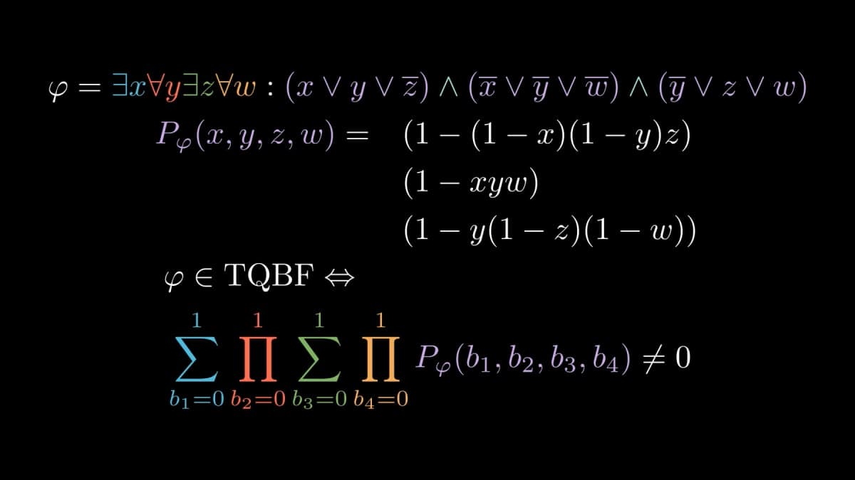
For example, the QBF $\varphi = \exists x \forall y \exists z \forall w : (x \vee y \vee \overline{z}) \wedge (\overline{x} \vee \overline{y} \vee \overline{w}) \wedge (\overline{y} \vee z \vee w)$

would get arithmetized as follows:

As a side note, I generated this animation using this tool I developed recently. At the end of the above visualization, we get:

Refinement of arithmetization

Before we can make use of the representation of QBF’s as polynomials in the interactive proof protocol, we need to ensure that they satisfy some “nice properties”. In this section, I will define such properties and show how we can ensure that they indeed hold. To make the notation introduced above more robust and easier to work with, we can first define the following functions that take a multivariate polynomial $p$ as input and produce another polynomial: $\begin{aligned} \exists_{x_i}(p)(x_1, \dots, x_n) &:= p(x_1, \dots, x_{i-1}, 0, x_{i+1}, \dots, x_n) + p(x_1, \dots, x_{i-1}, 1, x_{i+1}, \dots, x_n) \\ \forall_{x_i}(p)(x_1, \dots, x_n) &:= p(x_1, \dots, x_{i-1}, 0, x_{i+1}, \dots, x_n) \cdot p(x_1, \dots, x_{i-1}, 1, x_{i+1}, \dots, x_n) \\ Q_{x_i}(p) &:= \begin{cases} \exists_{x_i}(p) & \text{if } x_i \text{ is existentially quantified} \\ \forall_{x_i}(p) & \text{if } x_i \text{ is universally quantified} \end{cases} \end{aligned}$

The main equivalence we got above (as a result of arithmetization) can now be rewritten as follows: $\varphi \in \operatorname{TQBF} \Leftrightarrow Q_{x_1} Q_{x_2} \dots Q_{x_n} P_{\varphi} \neq 0$

From now on, I will call $Q_{x_i}$ a proof operator. The intuitive idea behind the interactive proof protocol we want to build is to check $Q_{x_1} Q_{x_2} \dots Q_{x_n}P_{\varphi} \neq 0$ by iteratively considering proof operators from left to right and in each step asking the prover to describe how the “behavior changes” using a univariate polynomial. As we will see below, this can be done in such a way so that the verifier can easily check whether what the prover sent “makes somewhat sense”, and if yes, then if the prover indeed lied, he will be forced with high probability to lie again and again, which leads to a high probability of the verifier finding out that the prover is dishonest at some stage — if the verifier catches the prover, he dismisses the alleged proof.

Linearization

For the polynomial-time verifier to be able to work properly with polynomials, we (will) need to ensure that they have low degree, i.e., the degree must itself be bounded by a polynomial in the size of $\varphi$. Note that the degree of $P_{\varphi}$ is low, because $\deg(P_{\varphi}) \le n \cdot m$, where $m$ is the amount of clauses. While $\exists_{x_i}$ adds polynomials which doesn’t increase their degree, $\forall_{x_i}$ multiplies polynomials meaning that the degree can get doubled in the worst case. If this happens in every step, then the degree of the entire arithmetization may get exponential, which is unacceptable. To resolve this issue, we can introduce a linearity operator $L_{x_i}$ defined as follows: $\begin{aligned} L_{x_i}(p)(x_1, \dots, x_n) &:= x_i \cdot p(x_1, \dots, x_{i-1}, 1, x_{i+1}, \dots, x_n) \\ &+ (1 - x_i) \cdot p(x_1, \dots, x_{i-1}, 0, x_{i+1}, \dots, x_n) \end{aligned}$

The idea is the following: $L_{x_i}$ outputs a polynomial that agrees with $p$ on all $x_1, \dots, x_n \in \{0,1\}$ such that the resulting polynomial is linear in $x_i$. For example, linearizing $xy^2+yx^2+x^3$ in $y$ $\begin{aligned} L_y(xy^2+yx^2+x^3) &= y \cdot (x + x^2 + x^3) + (1-y) \cdot x^3 \\ &= yx + yx^2 + yx^3 + x^3 - yx^3 \\ &= xy + yx^2 + x^3 \end{aligned}$

gives us $xy + yx^2 + x^3$ which is linear in $y$. The correctness of the linearity operator follows from the fact that $v^2 = v$ for all $v \in \{0, 1\}$. By composing multiple linearity operators, we can ensure that the polynomial is linear in all variables. Continuing the example above, we can linearize $xy + yx^2 + x^3$ in $x$ and obtain $\begin{aligned} L_x(L_y(xy^2+yx^2+x^3)) &= L_x(xy + yx^2 + x^3) \\ &= x \cdot (y + y + 1) + (1-x) \cdot 0 \\ &= 2xy + x \end{aligned}$

which agrees with $xy^2+yx^2+x^3$ on all inputs from $\{0, 1\}$. We can now sprinkle in linearity operators in the proof sequence $Q_{x_1} Q_{x_2} Q_{x_3} \dots Q_{x_{n-1}} Q_{x_n} P_{\varphi}$ as follows: $Q_{x_1} L_{x_1} Q_{x_2} L_{x_1} L_{x_2} Q_{x_3} L_{x_1} L_{x_2} L_{x_3} \dots Q_{x_{n-1}} L_{x_1} \dots L_{x_{n-1}} Q_{x_n} L_{x_1} \dots L_{x_n} P_{\varphi}$

Since we evaluate $P_{\varphi}$ only on binary values and the linearization operators guarantee that the outputted polynomial agrees with $p$ on all values from $\{0, 1\}$, it holds that $\begin{aligned} &Q_{x_{n-1}} L_{x_1} \dots L_{x_{n-1}} Q_{x_n} L_{x_1} \dots L_{x_n} P_{\varphi} = \\ &= Q_{x_1} L_{x_1} Q_{x_2} L_{x_1} L_{x_2} Q_{x_3} L_{x_1} L_{x_2} L_{x_3} \dots Q_{x_{n-1}} L_{x_1} \dots L_{x_{n-1}} Q_{x_n} L_{x_1} \dots L_{x_n} P_{\varphi} \end{aligned}$

which, in particular, implies that $\begin{aligned} \varphi \in \operatorname{TQBF} &\Leftrightarrow Q_{x_1} Q_{x_2} Q_{x_3} \dots Q_{x_{n-1}} Q_{x_n} P_{\varphi} \neq 0 \\ &\Leftrightarrow Q_{x_1} L_{x_1} Q_{x_2} L_{x_1} L_{x_2} Q_{x_3} L_{x_1} L_{x_2} L_{x_3} \dots Q_{x_{n-1}} L_{x_1} \dots L_{x_{n-1}} Q_{x_n} L_{x_1} \dots L_{x_n} P_{\varphi} \neq 0 \end{aligned}$

meaning that the problem of designing an interactive proof protocol for $\operatorname{TQBF}$ reduces itself to the problem of designing a protocol for showing that $Q_{x_1} L_{x_1} Q_{x_2} L_{x_1} L_{x_2} Q_{x_3} L_{x_1} L_{x_2} L_{x_3} \dots Q_{x_{n-1}} L_{x_1} \dots L_{x_{n-1}} Q_{x_n} L_{x_1} \dots L_{x_n} P_{\varphi} \neq 0$

Modular arithmetic

In the previous section, we’ve ensured that the intermediate polynomials all have low degree. However, there is another problem — we still may not be able to evaluate such low degree polynomials in polynomial time, because the value can get exponentially large with respect to the previous value, at every proof operator, meaning that the tight upper bound for the value of the entire polynomial is $O(2^{(2^n)})$. We can resolve this issue by picking a prime number $p$ and doing all computations modulo $p$, that is, in the $\mathbb{F}_p$ field. This doesn’t break any equivalence we have shown above, since there is a constant $d \in \mathbb{N}$ such that $\begin{aligned} &Q_{x_1} Q_{x_2} \dots Q_{x_n} P_{\varphi} \neq 0 \Leftrightarrow \\ &\Leftrightarrow\text{There is a prime } p \in O(2^{n^d}) \text{ such that } Q_{x_1} Q_{x_2} \dots Q_{x_n} P_{\varphi} \not\equiv 0 \mod p \end{aligned}$

holds. This is not hard to show using number theory — see Theorem 4 of Shamir’s paper for the details. Moreover, we can assume that $p > 2^n$ — this will be important for the correctness of the protocol that I will discuss at the end of this post.

Note that, as stated above, if $Q_{x_1} Q_{x_2} \dots Q_{x_n} P_{\varphi} \neq 0$, then the same statement will be true modulo at least one prime number $p$ that can be encoded using polynomially many bits. This does not mean that any prime $p > 2^n$ will work — the problem is that in the arithmetization polynomial we simulate $\exists$ quantifiers using a sum, but two non-zero values may become zero modulo $p$ once added together. For example, consider the formula $\varphi = \exists x \forall y \exists z \exists u \exists w : (x \vee \overline{z}) \wedge (\overline{z} \vee \overline{u} \vee \overline{w}) \wedge (\overline{x} \vee \overline{y} \vee \overline{u} \vee \overline{w}) \wedge (\overline{y} \vee \overline{z})$

with $n = 5$ variables. We could be tempted to just choose the first prime $p > 2^n = 32$, which is $p = 37$. Calculating the value of the arithmetizing polynomial gives us: $\begin{aligned} \forall_y \exists_z \exists_u \exists_w P_{\varphi} &= 5 \cdot x + 16 \\ \exists_x \forall_y \exists_z \exists_u \exists_w P_{\varphi} &= (5 \cdot 0 + 16) + (5 \cdot 1 + 16) \\ &= 16 + 21 = 37 = 0 \end{aligned}$

However, although $\exists_x \forall_y \exists_z \exists_u \exists_w P_{\varphi} = 0$ suggests that $\varphi \notin \operatorname{TQBF}$, $\varphi$ is actually a true sentence. This example illustrates why we need to be careful when choosing $p$.

Interactive protocol for TQBF

As mentioned earlier, the vague idea behind the protocol is to go over the operators from left to right and ask the the prover to describe “what has changed” using a polynomial. In the context of some polynomial $q(x_1, \dots, x_n)$ we now formalize this notion by defining the following univariate polynomial: $h_q(x_1) := \bigodot_{b_2=0}^1 \cdots \bigodot_{b_n=0}^1 q(x_1, b_2, \dots, b_n)$

Here, we assume without loss of generality that the variable of the first proof operator is $x_1$ (rename variables if this is not the case). Suppose we have some values $c, a_1, \dots, a_k \in \mathbb{F}_p$ and we want to check whether $g(a_1, \dots, a_k) = c$, where $g$ is a polynomial from the proof operator sequence, that is, $g(x_1, \dots, x_k) = Q_{x_1}(g'(x_1, \dots, x_k)), \quad Q_{x_1} \in \{\exists_{x_1}, \forall_{x_1}, L_{x_1}\}$

holds for some polynomial $g'$. This can be verified using the following interactive protocol, which I will refer to as the operator composition check protocol:

1. Verifier: If $k = 1$, set $s := g$, go directly to step 4 and accept if the check succeeded;
2. Verifier: Otherwise, ask the prover to send $h(x_1)$.
3. Prover: Sends $s(x_1)$ that is allegedly equal to $h(x_1)$.
4. Verifier: If $Q_{x_1} = \exists_{x_1}$, verify that $s(0) + s(1) = c$, if $Q_{x_1} = \forall_{x_1}$, verify that $s(0) \cdot s(1) = c$ and if $Q_{x_1} = L_{x_1}$, verify that $a_1 \cdot s(1) + (1 - a_1) \cdot s(0) = c$. If one of these checks failed, reject.
5. Verifier: Pick $a \in \mathbb{F}_p$ uniformly at random and re-run the same protocol to check that $s(a) = g'(a, a_2, \dots, a_k)$.

On top of this protocol, it is now easy to build the interactive proof protocol for $\operatorname{TQBF}$:

• Verifier: Ask the prover to send the value of the entire proof operator polynomial.
• Prover: Sends $c \in \mathbb{F}_p$,
• Verifier: If $c = 0$, reject (because this means that the prover directly confessed that the value of the polynomial is 0 meaning that $\varphi \notin \operatorname{TQBF}$).
• Verifier: Using the operator composition check protocol defined above, verify that

$Q_{x_1} L_{x_1} Q_{x_2} L_{x_1} L_{x_2} Q_{x_3} L_{x_1} L_{x_2} L_{x_3} \dots Q_{x_{n-1}} L_{x_1} \dots L_{x_{n-1}} Q_{x_n} L_{x_1} \dots L_{x_n} P_{\varphi} = c$

Example visualized

In this section I would like to present my tool that allows us to both obtain the interactive transcript in text format, as well as render a video animation showing in detail every aspect of the protocol. The implemented protocol is exactly the protocol defined in this post, all notations are also consistent. In the arithmetization section above, we have already arithmetized a concrete formula, namely $\varphi = \exists x \forall y \exists z \forall w : (x \vee y \vee \overline{z}) \wedge (\overline{x} \vee \overline{y} \vee \overline{w}) \wedge (\overline{y} \vee z \vee w)$

I will continue using this example formula. We obtain the following proof operator sequence: $\exists_x L_x \forall_y L_x L_y \exists_z L_x L_y L_z \forall_w L_x L_y L_z L_w P_{\varphi} = 1$

For this particular formula $\varphi$, the value of the polynomial will always be $1$ regardless of the choice of $p$, but from now on we will do all computations modulo $p = 17 > 16 = 2^n$. If we consider each operator in the above sequence separately and evaluate the part after that operator, then we obtain: $\begin{aligned} L_x \forall_y L_x L_y \exists_z L_x L_y L_z \forall_w L_x L_y L_z L_w P_{\varphi} &= 1 - x \\ \forall_y L_x L_y \exists_z L_x L_y L_z \forall_w L_x L_y L_z L_w P_{\varphi} &= 1 - x^2 \\ L_x L_y \exists_z L_x L_y L_z \forall_w L_x L_y L_z L_w P_{\varphi} &= -2 x y + x + 1 \\ L_y \exists_z L_x L_y L_z \forall_w L_x L_y L_z L_w P_{\varphi} &= -2 x y + x + 1 \end{aligned}$

Here, I have included only the first 4 polynomials. It follows that the prover must in the first round send $h(x_1) = 1 - x_1$ followed by $h(x_1) = 1 - x_1^2$ in the second round. Then the verifier will change the polynomial $g$ and assign a randomly chosen but fixed value to the $x$ variable. If, for example, the verifier chooses $x := a = 10$, then it means that in the third round the verifier would need to send $h(x_1) = (-2) \cdot 10 \cdot y + 10 + 1 = -3y - 6$. More generally, the $s = h$ polynomial the prover must send to be able to convince the verifier that $\varphi \in \operatorname{TQBF}$ is essentially the intermediate evaluation of the proof operator sequence, with values the verifier chose substituted for all variables except the current one. This is exactly the reason why it is essential that we ensure that the intermediate polynomials in the proof operator sequence all have low degree — otherwise the prover might not be able to come up with the $s = h$ polynomial of degree polynomial in the size of $\varphi$.

The following interactive transcript gets produces for $\varphi$, of which I am including only first 4 rounds here:

Working modulo prime p = 17
[V]: Asking prover to send value of the entire polynomial
[P]: Value = 1 =: c
------------------------------
Starting round 1. Current operator: E_{x}
[V]: Random choices: none
[V]: Asking prover to send s(x) = h(x)
[P]: Sending s(x) = 1 - x
[P]: deg(s(x)) = 1
[V]: s(0) + s(1) = 1, expecting to be equal to c = 1
[V]: Chose a = 13 for variable x
[V]: Random choices: x := 13
[V]: s(a) = 5 =: c
------------------------------
Starting round 2. Current operator: L_{x}
[V]: Asking prover to send s(x) = h(x)
[P]: Sending s(x) = 1 - x**2
[P]: deg(s(x)) = 2
[V]: a_1 * s_1 + (1 - a_1) * s_0 = 5, expecting to be equal to c = 5
[V]: Re-chose a = 10 for variable x (while linearizing it)
[V]: Random choices: x := 10
[V]: s(a) = 3 =: c
------------------------------
Starting round 3. Current operator: A_{y}
[V]: Random choices: x := 10
[V]: Asking prover to send s(y) = h(y)
[P]: Sending s(y) = -3*y - 6
[P]: deg(s(y)) = 1
[V]: s(0) * s(1) = 3, expecting to be equal to c = 3
[V]: Chose a = 10 for variable y
[V]: Random choices: x := 10, y := 10
[V]: s(a) = 15 =: c
------------------------------
Starting round 4. Current operator: L_{x}
[V]: Asking prover to send s(x) = h(x)
[P]: Sending s(x) = 1 - 2*x
[P]: deg(s(x)) = 1
[V]: a_1 * s_1 + (1 - a_1) * s_0 = 15, expecting to be equal to c = 15
[V]: Re-chose a = 15 for variable x (while linearizing it)
[V]: Random choices: x := 15, y := 10
[V]: s(a) = 5 =: c

And running the tool in rendering mode produces the following visualization of the protocol applied to $\varphi$:

The animation consists of the following parts:

• At the very top, the sequence of proof operators is located. In every round of communication, the proof operator corresponding to the beginning of the polynomial being considered, namely $g$, is highlighted with a yellow surrounding rectangle.
• Below the sequence of proof operators, the values that the verifier has assigned to variables so far, are displayed.
• In the center of the animation, the sequence of proof operators is visualized with a tree. This visualization allows us to very clearly see, in particular, the connection between $c$ and the sequence of proof operators, or, in other words, value of what part of the polynomial is currently being verified.
• In the bottom corners, the V and P stand for verifier and prover, respectively. Between these labels, the communication is visualized. In particular, it is visualized which messages both parties exchange and how the verifier checks that what the prover says is correct, in accordance with the protocol defined above.

Correctness of the protocol

Finally, to make the description of the protocol in this post complete, I would like to explain in my own words why the protocol defined above is correct. The completeness property of $\operatorname{IP}$ holds obviously — if $\varphi \in \operatorname{TQBF}$, then an honest prover will be able to convince the verifier no matter how the verifier tosses coins.

For the soundness analysis, we will first show the following lemma:

Lemma: Let $g$ be a polynomial, $c, a_1, \dots, a_k \in \mathbb{F}_p$ and suppose that we are checking whether $g(a_1, \dots, a_k) = c$ using the operator composition check protocol, but actually $g(a_1, \dots, a_k) \neq c$. Then the probability of either

• the verifier rejecting the proof in that very round (at step 4), or
• the verifier forcing the prover to continue lying in the next round, that is, re-running the protocol to verify $s(a) = g'(a, a_2, \dots, a_k)$ when it is actually the case that $s(a) \neq g'(a, a_2, \dots, a_k)$

is at least $1 - d/p$, where $d = \deg(h(x_1))$.

Proof: If the prover sends $s = h$, then, depending on the current proof operator, one of the checks in step 4 will fail and the verifier will therefore reject with probability $1 \ge 1-d/p$. On the other hand, if the prover sends $s \neq h$, then the polynomial $s(x_1) - h(x_1) \neq 0$ has degree at most $d$. This means that $s - h$ has at most $d$ roots, i.e., there exist at most $d$ values $a \in \mathbb{F}_p$ such that $s(a) = h(a)$. In other words, $\Pr[s(a) = h(a)] \le d/p$. Since the verifier uses the value $c = s(a)$ in the next round, it holds that $\Pr[s(a) \neq g'(a, a_2, \dots, a_k)] = \Pr[s(a) \neq h(a)] \ge 1 - d/p$

This completes the proof of the lemma.

Now suppose that $\varphi \notin \operatorname{TQBF}$. Then it is clear that the probability of the verifier not being fooled by the prover is at least the probability of the prover being forced to lie again and again, until he is either caught at some (possibly last) round. By applying the above lemma inductively, we get: $\Pr[\text{Verifier rejects or prover continues lying after } k \text{ rounds}] \ge \Big(1 - \frac{d}{p}\Big)^k$

Since $k \le 2 \cdot n^2 \in O(n^2)$, $p > 2^n$ and $d \le cn^c+c$ for some constant $c$, it holds that $\Pr[\text{Verifier rejects}] \ge \Big(1 - \frac{d}{p}\Big)^{2n^2} \ge \Big(1 - \frac{cn^c+c}{2^n}\Big)^{2n^2}$

We can calculate the limit of this probability using L’Hôpital’s rule: $\liminf_{n \to \infty}{\Pr[\text{Verifier rejects}]} \ge \lim_{n \to \infty}{\Big(1 - \frac{cn^c+c}{2^n}\Big)^{2n^2}} = 1$

By the definition of the limit, this means that for any $0 < \varepsilon \le 1$ there exists a fixed $n \in \mathbb{N}$ such that for all QBF sentences $\varphi$ with at least $n$ variables the probability of the verifier rejecting $\varphi \notin \operatorname{TQBF}$ is at least $1 - \varepsilon$. This in particular implies the soundness requirement of the $\operatorname{IP}$ complexity class, thus completing the proof of the correctness of the protocol.